Adverse Weather and Environmental Conditions: Rain, Snow, Fog, Night and Glare

FACT — AD-04 and AD-05 answered a sensor-centric question: “Under what conditions does the camera degrade? The radar? The LiDAR?” This lesson asks the same physics in reverse — an equally important engineering framing: “While it’s raining, which sensors remain reliable and how does the system adapt? While it’s foggy? At night?” Whether an automated driving system survives the real world depends not on any one sensor’s laboratory performance, but on the practical answer to these condition-centric questions.

In this lesson, you will learn:

1. The Inverse Framing — why a condition-centric view is a distinct, complementary engineering tool to a sensor-centric one.
2. Rain — camera contrast loss, LiDAR Mie attenuation, radar’s relative robustness, and wiper/washer coordination.
3. Snow — the total disappearance of lane markings, HD-map dependency, and accumulation on sensor housings.
4. Fog — the simultaneous collapse of camera AND LiDAR, and why radar becomes the “all-weather” backbone.
5. Night — why the active/passive sensor distinction matters for illumination dependence.
6. Glare — a genuinely unsolved problem for vision-only systems.
7. Summary Matrix — a sensor × condition reliability table.
8. The ODD Connection — why so many real-world ODDs explicitly exclude these conditions.

---

1. The Inverse Framing: A Condition-Centric View

AD-04/AD-05 Framing (Sensor-centric):           AD-25 Framing (Condition-centric):

  Camera → under what conditions does it fail?    Rain  → which sensor(s) remain reliable?
  Radar  → under what conditions does it fail?    Snow  → which sensor(s) remain reliable?
  LiDAR  → under what conditions does it fail?     Fog   → which sensor(s) remain reliable?
                                                   Night → which sensor(s) remain reliable?
                                                   Glare → which sensor(s) remain reliable?

INTERPRETATION — Both framings describe the same physical facts, but they feed different engineering decisions. The sensor-centric view is what you need when designing a sensor (which wavelength, which architecture); the condition-centric view is what you need when designing a fusion/decision architecture — because a real-time planner doesn’t ask “is my LiDAR degraded right now,” it asks “it’s foggy right now, how should I weight each sensor input.” This lesson works through each condition to answer that second question directly.

---

2. Rain

2.1 Camera: Contrast and Visibility Loss

Raindrops on the windshield act as tiny refractive lenses, bending light; residual water film and grime left by wipers add astigmatism-like blur. Beyond that, a rainy scene is intrinsically low-contrast — wet asphalt becomes more reflective (specular glare) while airborne droplets scatter background light. The result is a signal-quality drop that even the 120–140 dB HDR pipeline introduced in AD-04 §2.3 cannot fully compensate for.

2.2 LiDAR: Two Distinct Scattering Regimes

LiDAR range loss in rain has more than one root cause:

• Large raindrops (~0.5–5 mm diameter): Thousands of times larger than the LiDAR wavelength (905/1550 nm ≈ 1 µm), so their interaction with the beam is closer to geometric optics (refraction/reflection); each drop briefly deflects or blocks the beam.
• Fine mist/spray aerosol (~1–10 µm): Heavy rain throws up fine spray from the road surface and suspends micro-droplets at low altitude that sit squarely in the LiDAR wavelength’s own size range — this is where true Mie scattering (the physical principle introduced in AD-05) actually occurs. This aerosol layer scatters the laser pulse in all directions, both attenuating the returning signal and generating spurious backscatter echoes.

FACT — The practical consequence: as rain intensity increases, effective LiDAR range drops through two separate mechanisms at once — large-drop blocking and spray-aerosol Mie scattering; a LiDAR’s typical 200 m dry-weather range can fall below 100 m in a heavy downpour.

2.3 Radar: Relative Resilience

77–81 GHz radar wavelength (~4 mm) remains large relative to both raindrops and spray aerosol, so it largely retains the “all-weather” advantage covered in AD-04/AD-05. It is not fully immune, though: very heavy downpours (>50 mm/h) produce measurable atmospheric attenuation, and the dense spray cloud thrown up behind heavy vehicles raises the clutter floor on radar returns, complicating detection of low radar-cross-section (RCS) targets such as pedestrians and cyclists.

ASSUMPTION — Exact dB/km attenuation figures depend on precipitation rate, drop-size distribution, and radar frequency (76 vs 79 GHz); this lesson gives conceptual order-of-magnitude, and precise engineering budgets should reference the relevant radar supplier’s wet-weather test data.

2.4 Vehicle-Level Feedback: Wiper/Washer Coordination

The rain sensor (typically an infrared reflection sensor on the windshield) doesn’t just trigger the wiper — in modern architectures it also feeds back into camera detection confidence: the milliseconds during which the wiper blade sweeps across the lens are assigned a low-confidence flag for that frame (a brief “blind” window), and while washer fluid is being sprayed, camera input can be entirely down-weighted in the fusion layer until the next clean frame arrives. This is not a purely mechanical fix — it’s a feedback loop that reaches into the perception layer itself.

---

3. Snow

3.1 The Total Disappearance of Lane Markings: A Uniquely Hard Case

CRITICAL — Unlike every other degradation mode in this lesson (rain’s blur, fog’s contrast loss), snow doesn’t make lane detection harder — it removes the problem’s input entirely. In rain, a blurred lane-marking signal still exists; when a lane line is fully covered by a white blanket of snow, there is no edge left to detect, physically. This isn’t a case of the algorithm being “insufficient” — it’s a case where the ground-truth geometry to be detected is not present in the scene, even for a perfect perception system. A better neural network, a higher-resolution camera — neither can manufacture information that does not exist.

This is why lane-level localization under snow must shift from real-time lane detection to HD-map-based localization (see AD-08 — Localization: GNSS/RTK, Dead Reckoning, HD Maps and SLAM): the vehicle localizes itself against pre-mapped lane centerlines using GNSS-RTK + IMU + LiDAR point-cloud matching against fixed references snow doesn’t cover — curbs, poles, building facades. If the HD map is unavailable or its confidence is low, the only remaining safe option is graceful degradation or disengagement — the system must not attempt to “guess” the lane center, because a wrong guess gives the driver false confidence in the wrong direction.

3.2 Physical Accumulation on Sensor Housings

Snow and ice accumulating directly on the camera lens, LiDAR optical window, or radar radome blinds the sensor completely independent of algorithm performance — it is a purely mechanical/industrial design problem: light or waves simply cannot physically reach the surface. The real-world engineering solution is heated sensor covers — thin resistive heating wires embedded into camera and LiDAR windows (the same principle as a rear-window defroster) that keep surface temperature above freezing to prevent or melt snow/ice buildup. Radomes are generally not heated (material constraints exist to preserve RF transparency), but since wet snow/ice buildup can also attenuate radar signal, front-panel layout typically places the radar close to an already-heated zone (e.g., around the fog lamp, front grille).

3.3 Radar’s Relative Standing

Snowflakes (typically a few mm) are closer in size to the radar wavelength (4 mm) than raindrops are, producing a mild scattering effect; but as long as the radome stays clean, this is small compared to camera/LiDAR’s outright loss of vision. The critical variable is again physical blockage: if the bumper-mounted radar becomes covered in wet, compacted snow, RF transmissivity drops.

---

4. Fog

CRITICAL — Fog is the most instructive case study in this lesson because it makes AD-05’s “no sensor is reliable everywhere, hence fusion is mandatory” principle concrete and measurable: fog collapses camera AND LiDAR simultaneously, through the same physical mechanism.

Fog droplets’ typical diameter (1–10 µm) sits in the same order of magnitude as both visible light (400–700 nm) and LiDAR’s near-infrared wavelengths (905/1550 nm) — meaning both are squarely in the classic Mie scattering regime. For a camera, this means incoming light is scattered in all directions by airborne droplets (contrast collapses toward zero, a “white wall” appearance); for LiDAR, it means most of the emitted laser pulse is backscattered before it ever reaches the target, and range collapses dramatically.

The approximate relationship between Meteorological Optical Range (MOR — the distance at which a driver can distinguish a black object) and the atmospheric extinction coefficient (the Koschmieder/Kruse relation):

$\alpha \approx \frac{3.912}{V_{met}}$

where $V_{met}$ is meteorological visibility in meters and $\alpha$ is the extinction coefficient in 1/meter. The signal power an optical sensor (camera or LiDAR) receives falls off exponentially with distance traveled:

$I(R) = I_0 \cdot e^{-\alpha R}$

In dense fog with $V_{met} = 50\text{ m}$ ($\alpha \approx 0.078\text{ /m}$), a LiDAR pulse traveling 100 m out and back ($2R = 200\text{ m}$ total path) loses $e^{-0.078 \times 200} \approx e^{-15.6}$ of its signal — practically all of it.

Radar sits in a completely different regime: its wavelength (~4 mm) is roughly 400 times larger than a fog droplet’s diameter (~10 µm), placing it in the Rayleigh scattering regime (scattering efficiency scales as $(d/\lambda)^4$ — scattering becomes negligible as particle size shrinks relative to wavelength). Radar range is therefore almost entirely unaffected by dense fog — fog is the clearest proof of radar’s “all-weather” value.

Sensor	Fog Mechanism	Degree of Impact
Camera	Mie scattering (visible light, comparable to droplet size)	Very High
LiDAR	Mie scattering (NIR, comparable to droplet size)	Very High
Radar	Rayleigh scattering (λ ≫ droplet size)	Very Low

---

5. Night

5.1 The Operational Value of the Active/Passive Distinction

No condition makes the active/passive distinction introduced in AD-04 §1 more operationally decisive than night: radar and LiDAR carry their own illumination source — they operate entirely independent of ambient lighting. A radar chirp or laser pulse produces just as good a range/velocity measurement at pitch-black midnight as it does at high noon; the underlying physics doesn’t change at all.

A camera, by nature, depends on photons already present in the environment. Its night performance depends on two variables:

1. Sensor sensitivity: At low light, photon arrival is a statistical (Poisson) process, and SNR scales with the square root of the collected photon count ($\text{SNR} \approx \sqrt{N}$) — the relationship derived in AD-05 §1.2. Automotive cameras partially compensate with larger pixel wells, higher quantum efficiency, and noise-reduction ISP algorithms.
2. Scene illumination: Outside of headlights, streetlights, and oncoming traffic, there is no photon source in the scene; objects beyond headlight range (typically ~40–60 m on low beam, ~100–150 m on high beam) are practically invisible to a camera — whereas radar and LiDAR retain their own active range regardless of this limit.

INTERPRETATION — Some production designs attempt to close this asymmetry with active infrared illumination: near-IR emitters integrated into the headlight assembly light the scene in a band invisible to the human eye but visible to the camera, or a separate thermal (long-wave IR, ~8–14 µm) camera directly images human/animal body heat — this second approach is entirely independent of ambient light because it measures emitted heat rather than reflected light. But this complements the standard visible-light camera’s core limitation rather than eliminating it — it remains an optional, comparatively rare layer in most production ADAS suites.

5.2 Brief Blinding from Oncoming Headlights

A mechanism specific to night: an oncoming vehicle’s high beams can briefly saturate the camera’s dynamic range (the nighttime cousin of the glare physics covered in §6). Active sensors are immune to this because they distinguish the return of their own transmitted signal (via a specific frequency/phase signature) and are unaffected by a random external light source.

---

6. Glare

WARNING — A Genuinely Unsolved Problem — Direct low-angle sunlight entering the lens (sunrise/sunset, driving an east-west highway) is one of the few real failure modes for vision-reliant systems that remains without a complete engineering solution today.

The mechanism detailed in AD-05 §1.1 (instantaneous saturation of pixel full-well capacity → blooming → contrast collapse) reappears here, but it’s worth stressing why it remains unsolved: this is not an algorithmic failure — it’s a photonic limitation. Partial mitigations exist, but none is a complete fix:

• Lens coatings (anti-reflective/anti-glare): Reduce internal reflection (lens flare) within the lens elements, but cannot block a direct incoming ray.
• HDR pipeline (120–140 dB, AD-04 §2.3): Merges shadow and bright regions of a scene using separate exposures, but the direct solar ray entering the lens itself creates an optical scattering effect (a mechanism distinct from electronic saturation) that HDR cannot correct.
• Sun visor / mechanical shading: Works for a human driver, but cannot be directly applied to a fixed-position camera; some designs add a small hood to the camera housing, but it only covers a narrow angular range.
• Polarizing filters: Cut reflected light (especially off wet surfaces) by polarization, reducing glare, but have limited effect against direct solar rays and reduce overall light transmission (a disadvantage in low light).

INTERPRETATION — Glare remaining “unsolved” is the clearest case for why multi-modal sensing matters even for vision-forward approaches: the instant the sun temporarily blinds the camera, radar and LiDAR (both operating entirely outside the visible-light band) are wholly unaffected. We revisit this debate in AD-27 in the context of manufacturer philosophies (pure-vision vs multi-sensor).

---

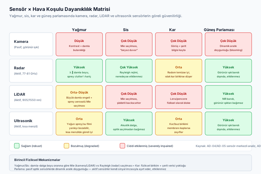
7. Summary Matrix: Sensor × Condition Reliability

Condition	Camera	Radar	LiDAR	Dominant Physical Mechanism
Rain	Low (contrast/droplets)	High (mild attenuation)	Low-Moderate (Mie + blocking)	Droplet size / wavelength ratio
Snow	Very Low (occlusion + lost lane data)	Moderate (if radome is clean)	Very Low (window/lens blocked)	Physical accretion + data absence
Fog	Very Low	Very High	Very Low	Mie (camera/LiDAR) vs Rayleigh (radar)
Night	Low-Moderate (illumination-dependent)	High (unaffected)	High (unaffected)	Active vs passive illumination dependence
Glare	Very Low	High (unaffected)	High (unaffected)	Dynamic range saturation

---

8. The ODD Connection: Why So Many Systems Explicitly Exclude These Conditions

As covered in AD-16 — Operational Design Domain (ODD): Definition, Taxonomy and Boundaries, an ADAS/AD system’s ODD carries explicit boundaries along the “Environmental Conditions” dimension — and each of the five conditions in this lesson is frequently and explicitly excluded in real production ODD definitions (“clear weather only,” “excludes dense fog/snow,” “visibility > 150 m”). This is not an admission of failure — it is honest engineering scoping: none of the physical mechanisms covered here (the absence of lane-marking data in snow, fog’s dual-modality collapse, glare’s photonic saturation) is fully solved by today’s sensor technology.

FACT — Seeing a “clear weather only” boundary in an ODD does not mean the system is poorly engineered — quite the opposite: a system that honestly defines its limits (and transitions to an MRM outside them) is far safer than one that claims unlimited capability but hasn’t actually been validated for it. A graceful degradation strategy (speed/following-gap restriction → L3-to-L2 fallback → MRM) operationalizes these honest limits instead of an abrupt all-or-nothing shutdown in adverse conditions.

---

Frequently Asked Questions (FAQ)

Q: If neither LiDAR nor camera can see lane markings in snow, how does the system stay in lane at all?

FACT — Because the system is no longer performing real-time perception; it’s determining its own position against a pre-built HD map (via GNSS-RTK + IMU + LiDAR point-cloud matching against fixed structures snow doesn’t cover — see AD-08). This is a switch to a different information source, not a “guess”; if the HD map itself is unreliable, the only safe option is graceful degradation.

Q: Isn’t radar alone sufficient in fog — why is camera/LiDAR still needed?

INTERPRETATION — Radar gives reliable range and velocity but has low angular resolution and cannot distinguish what an object is (a pedestrian vs. a trash can) (AD-04 §3, AD-06). Fog proves radar’s “all-weather” strength, but it cannot handle classification alone — the fusion architecture (AD-07) remains mandatory.

Q: Why aren’t heated sensor covers standard on every vehicle?

ASSUMPTION — Due to added power draw (typically on the order of several tens of watts per sensor), hardware cost, and complexity, this is generally found on higher-automation-tier systems or those targeting cold-climate markets; exact manufacturer implementations vary model to model.

---

Summary

• This lesson converts AD-04/AD-05’s sensor-centric degradation analysis into a condition-centric view: for each weather/illumination state, it answers “which sensor remains reliable, and how does the system adapt.”
• In rain, radar remains comparatively the most robust; camera loses contrast; LiDAR is attenuated through two distinct mechanisms — large-drop blocking and spray-aerosol Mie scattering.
• Snow is uniquely hard for lane detection because the ground-truth geometry to be detected is physically absent from the scene — the fix is HD-map-based localization or graceful degradation, not better real-time perception.
• Fog collapses camera and LiDAR simultaneously through the same Mie scattering mechanism while radar (in the Rayleigh regime) is nearly unaffected — the clearest concrete case for AD-05’s fusion-is-mandatory principle.
• Night sharpens the illumination-dependence gap between active (radar/LiDAR) and passive (camera) sensors; camera performance depends on sensor sensitivity and scene illumination, while active sensors depend on neither.
• Sun glare remains a generally unsolved problem for vision-reliant systems; partial mitigations exist (coatings, HDR, polarization) but no complete fix — underscoring the value of multi-modal sensing.
• Real production ODDs explicitly exclude most of these five conditions; this is honest engineering scoping, not a deficiency.

Sources and Verification Note

The physical mechanisms presented in this lesson draw on the “performance insufficiency” concept within the ISO 21448 (SOTIF) framework, ISO 26262 functional safety principles, SAE J3016 terminology, and Rasshofer, Spies & Spies’s work on the influence of weather phenomena on automotive laser radar systems. The Meteorological Optical Range (MOR) formula is the classical Koschmieder/Kruse atmospheric visibility relation. Numerical examples (range-loss percentages, attenuation coefficients) are intended to convey conceptual order of magnitude; exact values flagged ASSUMPTION should be verified against the relevant sensor supplier’s validated test data.

Next Lesson

• AD-26 — Global Regulations: UNECE, EU GSR II, US, China, Japan and Turkey: We now examine the legal counterpart to the environmental ODD boundaries covered here — which regulatory frameworks mandate which conditions, speed limits, and data-recording requirements, region by region.