AD-08 — Localization: GNSS/RTK, Dead Reckoning, HD Maps and SLAM

FACT — In AD-07 we saw the loose/tight coupling distinction in GNSS+IMU fusion and promised to go deeper on it here — this lesson delivers on that. But first we need to pin down a more fundamental question: exactly how is localization a different problem from perception?

In this lesson, we cover:

1. Localization vs. Perception: Why Do We Need Both?
2. GNSS-RTK: Centimeter-Level Position and Its Failure Modes
3. Dead Reckoning: IMU Double Integration and Quadratic Drift
4. HD Maps: What Makes a Map “HD”?
5. Map-Relative Localization: Landmark Matching with NDT/ICP
6. SLAM: Simultaneous Localization and Mapping
7. The Industry Philosophy Split: HD-Map-Dependent vs. Map-Light/Vision-First
8. Comparison Table: Localization Layers
9. FAQ, Summary, and Sources

---

1. Localization vs. Perception: Why Do We Need Both?

FACT — Perception tells the vehicle WHAT is around it, in an ego-centric reference frame: “there’s a car 20 m ahead,” “a cyclist is in my left lane.” Localization tells the vehicle WHERE IT ITSELF is, in an absolute or map-anchored reference frame: “the vehicle’s center of mass sits at this latitude/longitude, in the 2nd lane from the right, with a 0.03 rad heading offset from the lane centerline.”

These two pieces of information cannot substitute for each other. A planning layer (AD-10) may see the car ahead perfectly well through the camera, but if it doesn’t know which lane its OWN vehicle occupies, it cannot safely commit to a maneuver like “merge left from the right lane” — that decision depends on the vehicle’s absolute position on the map (which lane, how many meters to the intersection, whether the upcoming lane is closed). A localization system estimates the vehicle’s 6 Degree-of-Freedom (6-DoF) pose:

• Position: $[x, y, z]$ (latitude, longitude, altitude, or a local Cartesian frame)
• Attitude: $[\phi, \theta, \psi]$ (roll, pitch, yaw/heading)

FACT — A standard motorway lane is approximately $3.50\text{ m}$ wide, and a passenger car is roughly $1.90\text{ m}$ wide, leaving only $\sim 80\text{ cm}$ of margin on each side. Standard smartphone-grade GPS (with $3-5\text{ m}$ error) has an error dozens of times larger than that margin — nowhere near sufficient for automated driving. Industry consensus is that safe lane-level driving requires lateral position error below $10\text{ cm}$.

The four techniques covered in this lesson — GNSS-RTK, dead reckoning, HD map matching, and SLAM — are complementary layers that each try to reach this $10\text{ cm}$ target under different conditions; none is sufficient alone in every situation.

---

2. GNSS-RTK: Centimeter-Level Position and Its Failure Modes

RTK (Real-Time Kinematic) is far more precise than standard code-based (pseudorange) GNSS positioning because it measures the carrier wave’s PHASE:

1. A stationary ground base station, whose position is known to centimeter precision, compares the phase it measures for a given satellite against the expected phase, computing the delay introduced by the ionosphere/troposphere and satellite clock errors.
2. This correction stream (in RTCM format, typically delivered over a cellular link) is sent to the vehicle (the rover).
3. The vehicle subtracts this correction from its own carrier-phase measurement and resolves the integer wave-count ambiguity, bringing position error down to $1-2\text{ cm}$.

WARNING — RTK’s Achilles heel is the GNSS-domain reflection of the general principle we covered in AD-05: every sensor modality has a blind spot rooted in its own physics. For a camera that blind spot is line-of-sight occlusion; for radar it’s multipath propagation; for GNSS it’s the requirement of uninterrupted line-of-sight to at least 4 satellites:

• Urban canyons: Between tall buildings, direct signal is blocked while delayed reflections off building facades (multipath) mix with the direct signal, potentially shifting the fix by tens of meters.
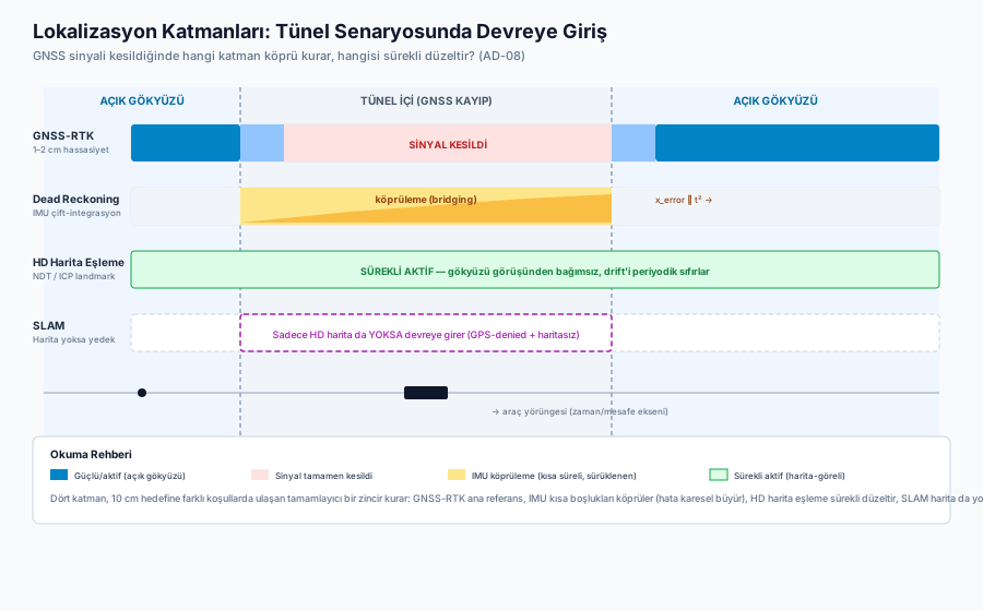
• Tunnels: Signal is lost entirely; the RTK fix collapses.
• Tree canopy, overpasses: Partial occlusion can drop visible satellite count below 4, making a 3D position fix impossible (we saw in AD-07 why this threshold is so critical in tightly-coupled EKFs).

These failure modes show that GNSS ALONE is insufficient for localization — some other technique must bridge the gaps.

---

3. Dead Reckoning: IMU Double Integration and Quadratic Drift

Dead reckoning is the bridging technique that keeps estimating vehicle motion from the last known position when GNSS is degraded or lost, by integrating IMU (accelerometer + gyroscope) and wheel-speed sensor data over time:

$v(t) = v_0 + \int_0^t a(\tau) \, d\tau, \qquad x(t) = x_0 + \int_0^t v(\tau) \, d\tau$

CRITICAL — Why does IMU-only dead reckoning drift over time? Accelerometer output is never perfect; it carries a small constant bias ($b_a$) plus thermal noise. Because this bias gets integrated TWICE over time ($a \to v \to x$), the resulting position error also compounds twice:

$x_{error}(t) \approx \frac{1}{2} b_a t^2$

Error grows QUADRATICALLY, not linearly with time — doubling $t$ quadruples the error. On top of this, the random-walk noise component of the sensor also accumulates through integration. The practical consequence: with a mid-grade automotive IMU and no GNSS correction, position error can open up to several meters within just a few tens of seconds. This is why dead reckoning is never an “infinite bridge” — it’s a temporary crutch that requires periodic re-anchoring, whether from GNSS signal returning, HD map matching providing a reference, or wheel odometry adding an extra constraint.

In practice, dead reckoning is therefore never “bare” IMU integration — it is continuously corrected either by the tightly-coupled GNSS+IMU EKF we saw in AD-07, or by the map matching covered in the next sections.

---

4. HD Maps: What Makes a Map “HD”?

FACT — A High-Definition (HD) map is QUALITATIVELY different from a phone navigation app’s road-level map (“this street runs this direction”). An HD map is a centimeter-scanned digital twin of the road, containing:

• Lane geometry: Centimeter-accurate spline/polynomial coordinates for every lane centerline, lane width, lane type (solid/dashed/HOV).
• Lane markings and curb positions: Exact 3D positions of painted lines, curb/sidewalk edges.
• Sign and signal positions: 3D coordinates of traffic lights and WHICH LANE each one governs (topological association), stop/yield sign positions.
• 3D landmark features: Poles, building facades, bridge abutments, retroreflective markers — fixed, repeatably recognizable structures that are the subject of the next section.

A standard navigation map says “this road exists, it runs this way”; an HD map says “this road’s 3rd lane centerline sits exactly HERE, to centimeter precision.” That difference turns the HD map into not just a route-planning input but also a localization reference — the topic of the next section.

---

5. Map-Relative Localization: Landmark Matching with NDT/ICP

The 3D landmark features carried by an HD map are the foundation of a technique fundamentally DIFFERENT from GNSS: map-relative localization. The idea is simple: the vehicle matches its live sensor data (LiDAR point cloud, camera imagery) against the same region in the pre-scanned HD map to correct its own position estimate — this is NOT an absolute reference from satellites, but a comparison against a previously known local reference.

1. ICP (Iterative Closest Point): Finds nearest-point correspondences between the live LiDAR point cloud and the previously scanned map point cloud, then iteratively computes the rotation/translation matrix that best fits the two.
2. NDT (Normal Distributions Transform): Rather than matching individual points, it divides space into small cells (e.g., $1\text{ m} \times 1\text{ m}$), converts each cell’s point distribution into a Gaussian probability density function, and aligns these continuous functions — considerably faster and more noise-robust than discrete point matching, which is why it’s often preferred over ICP for real-time driving.

INTERPRETATION — Map-relative localization’s big advantage over GNSS-RTK is that it does NOT depend on sky visibility — it can work in tunnels, urban canyons, even underground parking, because the reference is a previously scanned 3D structure, not satellites. Its cost is that the map must remain CURRENT: construction work, a new sign, or a repainted lane line can break the match — this is precisely the engineering cost at the center of the industry philosophy split discussed in Section 7.

---

6. SLAM: Simultaneous Localization and Mapping

One question remains unanswered: map-relative localization assumes the HD map already EXISTS — but how was that map built in the first place? Or what happens if the vehicle enters a region that has never been mapped (and where GNSS also doesn’t work)?

FACT — SLAM (Simultaneous Localization and Mapping) solves both problems AT THE SAME TIME: the vehicle BUILDS a map WHILE simultaneously using that (still-incomplete) map to estimate its own position. This is harder than it sounds because of a circular dependency: drawing an accurate map requires knowing where the vehicle is, but knowing where the vehicle is requires an accurate map. SLAM algorithms (e.g., Extended Kalman Filter SLAM, graph-based SLAM, particle-filter FastSLAM) solve this by jointly estimating both unknowns — map and pose — within a single probabilistic framework.

SLAM has two main practical uses:

• GPS-denied environments: In enclosed parking structures, tunnels, or dense urban zones where GNSS is unreliable and no HD map yet exists, the vehicle uses SLAM to simultaneously map its surroundings and localize within that map.
• Initial HD map production: An HD map doesn’t come from nowhere — someone has to build it FIRST. Dedicated mapping vehicles (equipped with survey-grade GNSS-RTK + IMU + multiple LiDARs) run SLAM-like techniques offline or semi-offline with much denser sensor data to produce the centimeter-accurate reference map, which then becomes the “previously known” reference that production vehicles use in the NDT/ICP matching of Section 5.

---

7. The Industry Philosophy Split: HD-Map-Dependent vs. Map-Light/Vision-First

The “the map must stay current” cost noted at the end of Section 5 sits at the center of a genuine, ongoing philosophy split in the autonomous driving industry:

INTERPRETATION — The HD-map-dependent approach (Waymo and most L4 robotaxi operators): every region the vehicle operates in is pre-scanned to centimeter precision by dedicated mapping vehicles and continuously kept up to date. The upside is very high precision and predictability (the vehicle “knows” the lane count around a blind curve, or that a lane 200 m ahead is closed, before ever perceiving it directly); the cost is that expanding into a new area requires an expensive mapping operation, and existing maps require ongoing maintenance (construction, sign changes, re-striped lanes) — this is one of the core engineering reasons Waymo operates in a limited number of cities, and within those cities, within pre-mapped zones.

The map-light/vision-first approach (the philosophy stated publicly by Tesla): real-time perception (especially camera-based deep learning, using techniques similar to the BEV fusion we covered in AD-07) re-derives lane geometry, sign/signal positions, and road topology on EVERY DRIVE; dependence on a pre-scanned centimeter-accurate HD map is minimized. The upside is much greater scalability (entering an unmapped road is not, in principle, a blocker); the cost is that real-time perception’s burden of working correctly EVERY TIME, under every condition (including the sensor limitations covered in AD-05), becomes far heavier.

Mobileye’s REM (Road Experience Management) concept is an example of a middle path between these two extremes: relatively cheap cameras on ordinary production vehicles (not dedicated mapping vehicles) collect LIGHTWEIGHT semantic landmark data (lane markings, sign positions — low-bandwidth features, not raw point clouds), which is aggregated from a large fleet in the cloud to keep the HD map continuously and cheaply up to date.

ASSUMPTION — The exact current technical details of the three approaches above (Waymo’s map update cadence, how much Tesla’s internal architecture still relies on an HD map, the exact data-collection protocol of Mobileye REM) are drawn from each company’s public technical presentations/blog posts and may change over time; the framework given here correctly reflects the general engineering trade-off but does not carry company-specific numerical claims.

---

8. Comparison Table: Localization Layers

Technique	Typical Accuracy	Operating Condition	Weakness	Role
GNSS-RTK	$1-2\text{ cm}$ (open sky)	Open sky, base station/correction stream available	Degrades/drops in urban canyons, tunnels, tree canopy	Primary absolute reference
Dead Reckoning (IMU)	Good for seconds, then degrades quadratically	SHORT bridging during GNSS outages	Unusable within minutes without re-anchoring	Short-term gap filling
HD Map Matching (NDT/ICP)	Centimeter-level, independent of sky visibility	Map pre-exists and is CURRENT	Mismatches if the map goes stale (construction, etc.)	Long-term, map-relative anchor
SLAM	Variable, depends on sensor quality	No pre-existing map, or GPS-denied region	High compute load; loop-closure errors can accumulate	Unmapped regions / initial map production

---

FAQ

Q: Can an automated vehicle drive at all without an HD map?

FACT — Yes, but in a more constrained, more reactive mode: it drives by tracking the lane lines it can see with the camera in the moment (the extreme end of the map-light philosophy in Section 7). An HD map lets the vehicle know the lane count around a blind curve, or a closed lane 200 m ahead, in ADVANCE, giving the planning layer (AD-10) much more lead time to react — it improves the safety margin but is not a strict prerequisite.

Q: Is GNSS without RTK correction completely useless?

INTERPRETATION — No; uncorrected standard GNSS ($3-5\text{ m}$ error) is still useful at a coarse “which street/which direction” level and provides a coarse starting point (a prior) for dead reckoning or HD map matching. But for lane-level ($<10\text{ cm}$) accuracy, RTK correction (or an equivalent map-relative technique) is practically mandatory.

Q: Can SLAM completely replace GNSS-RTK?

ASSUMPTION — In theory SLAM alone can map an environment and localize within it, but in practice a SLAM map produced without an absolute geographic anchor (tying the map to real-world coordinates) is prone to drift — especially cumulative error and loop-closure error over long routes. In industry, SLAM is used less as a replacement for GNSS-RTK and more to fill the gaps where it doesn’t work, and to feed initial map production — this is a generalization drawn from current public engineering practice and may vary by company.

---

Summary

• Localization estimates where the vehicle ITSELF is (absolute/map-anchored); perception estimates WHAT is around it (ego-centric) — planning needs both.
• GNSS-RTK delivers $1-2\text{ cm}$ accuracy under open sky but degrades or drops in urban canyons and tunnels — the GNSS-domain reflection of the principle that every sensor has its own physical blind spot (AD-05).
• Dead reckoning bridges GNSS gaps via IMU double integration, but constant-bias error grows QUADRATICALLY ($x_{error} \propto t^2$) — periodic re-anchoring is mandatory.
• HD maps are digital twins carrying centimeter-accurate lane geometry plus 3D landmark features; those landmarks are the foundation of map-relative localization via NDT/ICP.
• SLAM jointly solves mapping and localization when no map exists or in GPS-denied regions; it is used both as real-time fallback and for producing the initial HD map.
• The industry’s HD-map-dependent (Waymo) and map-light/vision-first (Tesla) philosophies are a genuine, ongoing engineering debate over the precision/scalability trade-off; Mobileye’s REM crowdsourced mapping is a middle path between the two extremes.

Sources and Verification Note

The localization framework in this lesson draws on: Thrun, Burgard & Fox — Probabilistic Robotics (Bayesian filtering, the probabilistic foundations of SLAM); Groves — Principles of GNSS, Inertial, and Multisensor Integrated Navigation Systems (GNSS-RTK, IMU drift dynamics); Levinson & Thrun — Robust Vehicle Localization in Urban Environments Using Probabilistic Maps (map-relative localization, NDT-based matching); Szeliski — Computer Vision (point-cloud registration geometry). Company-specific architecture claims (Waymo/Tesla/Mobileye’s exact current implementations) are drawn from public technical presentations, may change over time, and are therefore marked as ASSUMPTION.

Next Lesson

• AD-09 — Prediction: Intent Estimation and Probabilistic Trajectory Forecasting: This lesson covered how the vehicle knows its OWN position — AD-09 covers how we forecast where OTHER agents (vehicles, pedestrians, cyclists) around it will be over the next few seconds.