
- Explain the physical foundations and inputs/outputs of the lateral (steering) and longitudinal (throttle/brake) vehicle control loops.
- Analyze geometric trajectory-tracking algorithms such as Pure Pursuit and Stanley.
- Formulate PID control as the simplest classical approach and identify its weaknesses.
- Understand how Model Predictive Control (MPC) works and why it outperforms PID.
- Evaluate the additional challenge regenerative/friction brake blending poses for the control layer in EVs.
- Explain why control loops run at a much higher frequency than perception/planning.
AD-11 — Vehicle Control: Lateral/Longitudinal Control and Trajectory Tracking
FACT — The motion planner we examined in AD-10 produces, every cycle, a continuous, jerk-optimal, collision-free trajectory: . But this trajectory is a geometry on paper — it isn’t what moves the vehicle. The Vehicle Control layer is the final link in the planning hierarchy: it takes this geometric/kinematic trajectory and converts it into concrete, millisecond-scale commands sent to real actuators (the steering motor, throttle/torque request, brake pressure).
In this lesson we’ll examine the two independent sub-problems of the control layer — lateral and longitudinal control — starting from classical geometric methods, moving through PID, and arriving at Model Predictive Control (MPC), the industry standard in production:
- The Final Task of the Control Layer
- Lateral Control — Geometric Methods: Pure Pursuit and Stanley
- Lateral Control — PID: The Simplest Classical Approach
- Lateral Control — Model Predictive Control (MPC)
- PID or MPC? Why Production Favors MPC
- Longitudinal Control: Throttle/Brake Blending
- A Special Challenge in EVs: Regenerative/Friction Brake Blending
- Why Does the Control Loop Run Much Faster Than Perception/Planning?
- End-to-End Example: Turning a Lane-Change Trajectory into Actuator Commands
- Notes from Real Systems
1. The Final Task of the Control Layer
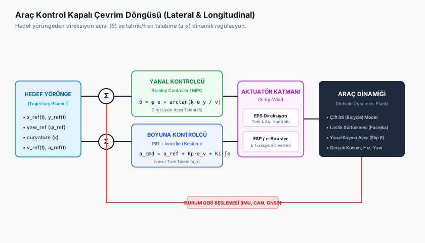
FACT — The control layer takes the reference trajectory handed down by the motion planner, , and solves it by splitting it into two independent sub-problems:
| Sub-Problem | Input | Output (Actuator Command) | Physical Actuator |
|---|---|---|---|
| Lateral Control | Reference path geometry , current position/heading | Steering angle | EPS (Electric Power Steering) motor |
| Longitudinal Control | Reference speed/acceleration , current speed | Acceleration/deceleration request | Torque request (inverter) + brake pressure (ESP/iBooster) |
This split is the natural continuation, at the control layer, of the Frenet decoupling (–) we saw in AD-10: longitudinal and lateral dynamics can be controlled largely independently at low-to-moderate speeds (this independence weakens at high speed and near dynamic limits — see Section 4).
INTERPRETATION — Most controllers represent the vehicle with a simplified bicycle model: instead of four wheels, the front and rear axles are each modeled as a single wheel, establishing a geometric relationship between wheelbase , heading, and steering angle. This simplification works very well at low-to-moderate speeds; at high speed and on slippery surfaces, dynamic models that account for tire slip angle become necessary (Section 4).
2. Lateral Control — Geometric Methods: Pure Pursuit and Stanley
The oldest and simplest lateral controllers derive a steering angle directly from the vehicle’s bicycle-model geometry; they require no dynamics model or optimization.
Pure Pursuit: Fits a circular geometric arc from the vehicle’s rear axle center to a predetermined “lookahead point” on the reference trajectory:
where is the wheelbase, is the angle between the vehicle’s current heading and the lookahead point, and is the lookahead distance. The lookahead distance is typically scaled dynamically with speed (): a short lookahead at low speed gives precise tracking, while a longer lookahead at high speed prevents oscillation (zigzagging).
Stanley Controller: References the front axle center instead, and decomposes the error into two components — heading error (the angle difference between the vehicle’s heading and the path tangent) and cross-track error (the perpendicular distance from the front axle to the path):
EXAMPLE — Because the second term of the Stanley formula has in the denominator, it produces a very aggressive correction at low speed (e.g. during a parking maneuver) and becomes mathematically undefined as ; in practice is clamped to a small lower bound ().
Both of these methods are geometric: they don’t model the vehicle’s mass, tire-road friction, or actuator rate limits in any way — they simply give a kinematic answer to “where should I be right now.”
3. Lateral Control — PID: The Simplest Classical Approach
As an alternative to the geometric methods, the lateral error can be fed directly into a PID (Proportional-Integral-Derivative) controller — control engineering’s most common and simplest classical tool:
where is typically the cross-track error (, defined as in Section 2). The three terms each use a different piece of information:
- Proportional (): An instantaneous correction proportional to the current error — a large error produces a large response.
- Integral (): Compensates for error accumulated over time — e.g. zeroes out a systematic bias caused by a persistent lateral force like wind or road camber (“steady-state error”).
- Derivative (): Responds to the rate of change of the error — if the error is closing quickly, it applies a braking effect to damp overshoot and oscillation.
CRITICAL — PID is conceptually incomplete for trajectory tracking: it only reacts to the current error (and its history/derivative), it never looks ahead at the curvature of the upcoming road. At the start of a curve, PID waits until error has already built up before it responds — producing a delayed, reactive correction. PID also cannot incorporate actuator constraints (maximum steering angle/rate) or the vehicle dynamics’ nonlinear limits (tire slip limit) into the model at all — these constraints can only be “managed” indirectly, by tuning the gains () conservatively by hand to stay on the safe side.
4. Lateral Control — Model Predictive Control (MPC)
FACT — In production autonomous driving stacks, the industry standard for lateral (and often longitudinal) control is Model Predictive Control (MPC). MPC’s core idea is fundamentally different from PID’s: it corrects error not by looking backward, but by predicting the future.
At each control cycle (typically every ), MPC runs the following steps:
- Using the vehicle’s current state () and a vehicle dynamics model (a bicycle model plus tire slip angle, — in the spirit of the dynamic modeling approach in lessons like MOTOR-19), it simulates possible future trajectories over a horizon of several seconds for different candidate control-input sequences ().
- It scores each candidate trajectory with a cost function based on how well it tracks the reference trajectory, control effort, and constraint violations:
- It solves this constrained optimization problem (typically a quadratic program) to find the best control sequence, but applies only the first element of the sequence ().
- On the next cycle, starting from the newly measured state, it repeats the entire process from scratch (the receding-horizon principle) — this way model errors and unforeseen disturbances are continuously corrected.
EXAMPLE — If MPC’s horizon is, say, a 2-second window with steps (100 time steps), each cycle evaluates dozens of candidate steering-angle sequences (each with its own predicted future trajectory); the lowest-cost sequence is selected, only its first command is applied, and the rest is discarded.
5. PID or MPC? Why Production Favors MPC
MPC’s advantage over PID rests on three concrete reasons:
- It models constraints natively: MPC writes physical/safety constraints — maximum steering angle, maximum steering angle rate of change (), tire slip limits — directly into the optimization problem itself. In PID, these constraints can only be “hoped for” via indirect, trial-and-error gain tuning.
- It sees the future: Because MPC directly incorporates the curvature of the road ahead (future points of the reference trajectory) into its optimization, it can begin turning the wheel before a curve even starts — whereas PID waits until error has already appeared.
- It handles coupled dynamics: At high speed, lateral and longitudinal dynamics are not independent (e.g. braking shifts load onto the front axle, changing tire grip). MPC can model both channels — or their interaction — within the same optimization framework, while two separately tuned PID loops cannot inherently see this interaction.
WARNING — MPC’s cost is computational: a real-time constrained optimization problem must be solved every cycle. Unlike PID’s simple arithmetic operation, this requires deterministic real-time solvers on production ECUs and careful management of the computational budget — MPC’s spread across production stacks has been made possible in part by automotive-grade processors becoming capable of absorbing this cost.
Geometric methods (Pure Pursuit, Stanley) remain in use for low-speed, low-risk scenarios (e.g. parking assist, low-speed urban L2) because they’re computationally cheap and sufficiently stable there; MPC is the preferred approach at highway speeds and in higher-responsibility (L3+) systems.
6. Longitudinal Control: Throttle/Brake Blending
The longitudinal controller continuously blends throttle (torque request) and brake pressure to track the target speed/acceleration profile handed down by the planner ():
- If the target acceleration : a torque request is sent to the motor/inverter (see MOTOR-20 — cascaded torque/speed/current loops).
- If the target acceleration : the brake system engages (a pressure request through an electronic brake actuator such as ESP/iBooster).
- Around : the system must transition between throttle and brake without hunting — this transition zone is usually managed with a small dead-band and a smoothing filter; otherwise the vehicle would oscillate continually between throttle and brake, creating an uncomfortable ride.
The longitudinal controller is also typically implemented as a PID (in simpler implementations) or as the longitudinal channel of the MPC (in advanced implementations, part of the same optimization framework from Section 4).
7. A Special Challenge in EVs: Regenerative/Friction Brake Blending
CRITICAL — On the brake side, longitudinal control in electric vehicles contains an extra layer that isn’t present in internal-combustion vehicles: a negative torque request can be met by two different physical mechanisms — regenerative braking, which puts the electric motor into generator mode and recovers kinetic energy back into the battery, and classical friction braking (disc/drum). The transition between these two must be smooth, both for comfort and for safety.
Factors that complicate this blending:
- Regen capacity is not constant: when battery state of charge (SOC) is high, or temperature is too low/high, the battery’s charge-acceptance limit drops, and the available regenerative torque can drop suddenly — in that case the controller must instantly and imperceptibly hand off the shortfall in deceleration torque to friction braking (see MOTOR-27 — regenerative braking and power limits).
- Timing precision: when ABS/ESP detects wheel slip (requiring rapid intervention on icy/wet surfaces), regenerative torque must be cut and handed off to friction braking very quickly — this transition typically has a time budget on the order of tens of milliseconds.
- Comfort: if the torque transition between the two brake sources is abrupt, the passenger feels a noticeable jerk (see AD-10 Section 6); transition ramps and anti-jerk damping filters (see MOTOR-20) are therefore integrated into the longitudinal control loop.
INTERPRETATION — This blending becomes even more prominent in one-pedal driving modes: for the deceleration felt when the accelerator is released to stay consistent, the total deceleration torque must be held constant — friction braking supplementing as needed — even as regenerative capacity fluctuates; the driver should never be able to feel which mechanism is actually active.
8. Why Does the Control Loop Run Much Faster Than Perception/Planning?
FACT — The perception, prediction, and motion-planning layers we saw in AD-09 and AD-10 typically run at , while the control loop runs at a much higher frequency — typically .
This is a direct consequence of the control layer’s role in the system — it is the last line of defense:
- The trajectory produced by the planning layer can already be stale by the time it’s used (until the next planning cycle) — during that time the vehicle has moved, and small disturbances like wind or road camber may have appeared.
- The control loop continuously re-measures and corrects for this slightly stale reference at high frequency; the planning layer determines the “overall strategy” (what to do), while the control layer determines “how to execute it given the current reality.”
- The control loop also has to operate close to the actuators’ own internal control bandwidth (EPS motor, brake actuator) — a low-frequency command stream cannot make efficient use of the actuators’ physical response speed and produces delayed, jerky motion.
WARNING — Control loop frequency is not a comfort preference, it’s a safety requirement: a controller that doesn’t run at a high enough frequency can turn even a small delay into a large position error at high speed (at , a delay corresponds to roughly of additional travel).
9. End-to-End Example: Turning a Lane-Change Trajectory into Actuator Commands
Let’s continue the lane-change scenario from AD-10 Section 8 — the motion planner produced a lateral trajectory and a longitudinal profile with mild acceleration. The control layer processes this as follows:
| Step | Input | Controller | Output |
|---|---|---|---|
| Lateral | Reference , current heading/speed | MPC (at highway speed, ) | Steering angle command , updated every |
| Longitudinal | derived from reference | Longitudinal PID/MPC | Small positive torque request (mild acceleration during the maneuver) |
| Result | — | — | The EPS motor smoothly turns the wheel, the inverter applies a small extra torque; the vehicle completes a lane change faithful to the plan and jerk-optimal, in |
This loop repeats tens of times per second throughout the maneuver; each repetition compares the vehicle’s actual position against the reference trajectory and instantly corrects small deviations.
10. Notes from Real Systems
ASSUMPTION — The exact internal architecture of production vehicle control stacks (gain tables, MPC horizon lengths, solver choices) is generally not public; the notes below rely on publicly available academic/technical sources.
- Mobileye’s EyeQ system-on-chip family, supplied to multiple OEMs, serves as a reference point not just for generating perception output but also, in some ADAS functions (e.g. LKA, covered in AD-12), for producing lateral control commands; the exact control algorithm chosen (geometric/PID/MPC) varies by OEM and function (marked ASSUMPTION since specific internal details are not fully public).
- In academic and open-source stacks (e.g. Autoware, Apollo), both geometric methods (Pure Pursuit, Stanley) and MPC-based controllers exist together as reference implementations; geometric methods are preferred for low-speed/simple scenarios, MPC for highway/high-speed scenarios.
- Regenerative/friction brake blending can also be supported by a separate “brake feel simulator” hardware, so that the pedal feel stays consistent — the resistance the driver feels when pressing the pedal is kept constant regardless of which brake mechanism is actually working in the background.
Frequently Asked Questions (FAQ)
Q: Is PID no longer used at all?
No — PID is still widely used in longitudinal control (in one-dimensional, less-constrained problems like speed tracking) and in low-risk/low-speed lateral control scenarios; its simplicity, low computational cost, and ease of verification still make it attractive. MPC’s advantage becomes pronounced specifically in scenarios with high speed, tight constraints, and coupled dynamics.
Q: What happens if MPC’s prediction model is wrong?
Model error (e.g. the tire-road friction coefficient being lower than assumed) degrades MPC’s performance, but because of the receding-horizon principle — the state is re-measured and the optimization is re-run from scratch every cycle — error doesn’t accumulate: MPC continuously self-corrects. Still, significant model error may require tightening safety margins.
Q: How does the control loop handle an actuator failure?
The control layer typically monitors actuator feedback (actual steering angle achieved, actual brake pressure achieved); if a persistent discrepancy is detected between the commanded and achieved value, this is treated as a fault signal and the system transitions to a safe state (e.g. handover to the driver, emergency deceleration) — this is usually the responsibility of a separate safety-monitoring layer.
Summary
- The control layer is the final and highest-frequency link in the hierarchy, converting the planning layer’s geometric trajectory into steering angle and throttle/brake commands.
- For lateral control, geometric methods (Pure Pursuit, Stanley) are simple and computationally cheap; PID is the simplest classical feedback approach but cannot see the future or natively model constraints.
- MPC fixes both of PID’s weaknesses by predicting multiple future trajectories with a vehicle dynamics model each cycle and selecting the best one under constraints; its cost is real-time optimization overhead.
- Longitudinal control tracks target speed/acceleration via throttle/brake blending; in EVs, the smooth transition between regenerative and friction braking is an added engineering challenge.
- Control loops () run much faster than perception/planning () because control is the safety-critical last line, making real-time corrections against a slightly stale plan.
Sources and Verification Note
This lesson is based on Rajamani’s (Vehicle Dynamics and Control) classical vehicle dynamics/control framework, on the control-prediction relationship discussed in Thrun et al. (Probabilistic Robotics), and on the output format that Werling et al.’s Frenet-based trajectory generation hands off to the control layer. Notes on EyeQ and the internal architecture of production stacks are based on publicly available technical sources and are marked ASSUMPTION; ISO 26262 and ISO 21448 are the reference standards for the control layer’s functional safety and “safety of the intended functionality” (SOTIF) requirements. The lastVerified date is the date of this lesson’s last technical review.
Next Lesson
- AD-12 — Core ADAS Features: AEB, ACC, LKA, LCA, BSD, RCTA and TSR: We’ll see how the control layer covered in this lesson turns into concrete ADAS features in production vehicles (emergency braking, adaptive cruise control, lane keeping), along with their sensor requirements and triggering logic.
Technical Diagrams
Quiz
Which vehicle actuator is primarily governed by lateral control loops?
Lateral control commands the steering system to track road curvature and lane centerlines.
How should lookahead distance in a Pure Pursuit controller scale with vehicle velocity?
Lookahead distance scales with speed ($L_d = k \cdot v$) to ensure high-speed dynamic stability.
Which two fundamental error metrics does the Stanley lateral controller simultaneously resolve?
Stanley steering control reconciles heading error against front-axle cross-track error.
Why is Model Predictive Control (MPC) favored over geometric trackers during high-speed cornering?
MPC handles multi-variable dynamics, tire non-linearities, and strict physical actuator rate limits.
What is the primary benefit of acceleration Feedforward in longitudinal vehicle velocity regulation?
Feedforward commands target inertial acceleration directly, suppressing steady-state tracking lag.
Glossary
| English Term | Definition |
|---|---|
| Dynamic Driving Task (DDT) | All the real-time operational (steering, braking, accelerating) and tactical (lane changes, gap selection, object avoidance) functions required to operate a vehicle in on-road traffic. |
| Time-to-Collision (TTC) | The remaining time in seconds before two vehicles collide if their relative speed and heading remain unchanged (TTC = relative_distance / relative_velocity). |