AD-10 — Planning: Route, Behavior and Motion/Trajectory Planning

FACT — The perception and prediction layers of an autonomous driving stack answer “what’s around me, and what will it do?” (see AD-09). The Planning layer must answer an entirely different question: “What should I do right now?” This question spans too wide a range of timescales and complexity to be solved by a single algorithm — from a minutes-scale decision like “which highway should I take” down to a hundreds-of-milliseconds decision like “exactly how many degrees should I turn the wheel right now.”

In this lesson we examine the three-layer architecture that manages this range, the mathematical tools of each layer, and how they chain together in a lane-change maneuver:

1. The Planning Hierarchy: A Three-Layer Architecture
2. Layer 1 — Route / Mission Planning
3. Layer 2 — Behavior Planning
4. Layer 3 — Motion / Trajectory Planning
5. The Frenet Coordinate Frame: Why $[s, d]$ Instead of $[x, y]$?
6. Jerk Minimization and Quintic Polynomials
7. Cost Function and Trajectory Selection
8. End-to-End Example: Changing Lanes to Pass a Slow Vehicle
9. Notes from Real Systems

---

1. The Planning Hierarchy: A Three-Layer Architecture

FACT — Planning in autonomous driving is not solved as a single monolithic optimization problem; to keep computational complexity manageable, nearly every production and research stack splits it into a three-layer hierarchy. Each layer takes the previous layer’s output as input and narrows the horizon it inherits:

Layer	Time Horizon	Input	Output	Typical Algorithm Family
Route / Mission	Minutes – hours	Road network graph, points A and B	Ordered list of road/lane segments	Graph search (A*, Dijkstra)
Behavior	Seconds – tens of seconds	Traffic state, lane options, upcoming exit	Discrete high-level maneuver decision	State machine, decision tree, (PO)MDP
Motion / Trajectory	Hundreds of ms – a few seconds	Selected maneuver + obstacles + vehicle dynamics	Continuous geometric path + speed profile	Frenet lattice, quintic polynomial, optimization

The reason for this split is pure engineering pragmatism: the question “what’s the shortest route from Istanbul to Ankara,” the question “should I merge into the right lane right now,” and the question “exactly where should I point the wheels over the next 2 seconds” require very different data structures and very different update frequencies. Trying to merge them into a single layer would be both computationally infeasible and would make debugging impossible.

---

2. Layer 1 — Route / Mission Planning

Route planning is conceptually very similar to the problem consumer navigation apps (Google Maps, Waze) solve, but it operates integrated into the autonomous driving stack: its output is not a flat list of streets but a lane-level HD-map graph path (including which lane to stay in and which lane to move to at which intersection).

The road network is modeled as a weighted graph $G = (V, E)$ whose nodes are intersections/lane-segment endpoints and whose edges are drivable lane segments. The cost of each edge is typically a weighted sum of:

$w(e) = \alpha \cdot t_{travel}(e) + \beta \cdot d_{distance}(e) + \gamma \cdot c_{road\_class}(e) + \delta \cdot c_{traffic}(e)$

The A* algorithm narrows the search space by adding an admissible heuristic $h(n)$ — one that never overestimates the remaining distance to the goal — to Dijkstra’s $g(n)$ (the true cost so far from the start):

$f(n) = g(n) + h(n)$

INTERPRETATION — The route planning layer is generally a “coarse” solution and is recomputed only a handful of times over the course of a trip (traffic changes, a missed exit). The two layers below it, in contrast, re-run tens of times per second — further evidence of why these need to be separate layers.

---

3. Layer 2 — Behavior Planning

Once the route layer has provided “which sequence of lanes to follow,” the behavior planner is responsible for tactically executing that route within real traffic: stay in lane, change lanes left, slow down when approaching a vehicle ahead, yield at an intersection, stop for a pedestrian.

The most common practical implementation is the Finite State Machine (FSM):

                 gap_sufficient & signal_on
   ┌──────────┐ ─────────────────────────► ┌────────────────────┐
   │ LANE_KEEP│                            │ PREPARE_LANE_CHANGE │
   └──────────┘ ◄───────────────────────── └────────────────────┘
        ▲            gap_lost                        │ gap confirmed
        │                                            ▼
        │                                   ┌──────────────────┐
        └────── maneuver complete ────────── │ EXECUTE_LANE_CHG │
                                              └──────────────────┘
        ▲
        │  obstacle_detected (TTC < threshold)
   ┌──────────────┐
   │ EMERGENCY_STOP│
   └──────────────┘

Transition criteria typically include: the safety gap in the target lane ($gap > gap_{min}$, itself a function of the target lane vehicle’s speed and the ego vehicle’s speed), relative speed difference, and the maneuvers currently permitted by the Operational Design Domain (ODD).

CRITICAL — Pure FSMs are simple and verifiable, but they cannot naturally represent the uncertainty inherent in real traffic (another driver’s intent is never certain — see AD-09). This is why more sophisticated stacks model the behavior layer as a decision process (Markov Decision Process / Partially Observable MDP): each discrete maneuver option is an action, traffic state is a state, and the selection is made via a reward function that maximizes the trade-off between safety/legality/comfort/progress. The FSM is a deterministic, easy-to-verify special case of this more general framework, used widely in practice.

The behavior layer’s output is always discrete and high-level — it says “change lanes left,” but it never says “turn the wheel 3.2 degrees.” That final step is delegated to a lower layer.

---

4. Layer 3 — Motion / Trajectory Planning

The motion planner converts the discrete decision handed down by the behavior planner (e.g. “change lanes left”) into a continuous trajectory that the vehicle’s actuators can physically execute:

$\xi(t) = \left[ x(t),\ y(t),\ v(t),\ a(t) \right], \quad t \in [0, T]$

This trajectory must satisfy the following constraints simultaneously:

• Kinematic constraints: maximum curvature $\kappa(t) \le \kappa_{max}$ (the tightest radius the vehicle can turn), maximum longitudinal/lateral acceleration $|a(t)| \le a_{max}$.
• Comfort constraints: maximum jerk — see Section 6.
• Obstacle constraints: the trajectory must not intersect the predicted positions of other vehicles/pedestrians (see AD-09) at any time $t$.
• Legal/map constraints: lane boundaries, speed limit, traffic light state.

This layer is re-run tens of times per second (typically $10\text{–}20\ \text{Hz}$), because the previous trajectory can become invalid both as the vehicle moves and as the behavior of other traffic participants is updated.

---

5. The Frenet Coordinate Frame: Why $[s, d]$ Instead of $[x, y]$?

FACT — In a Cartesian coordinate system ($x, y$), even expressing a simple constraint like “stay in lane” on a curving road requires a complicated, road-dependent nonlinear equation — because the concept of “lane” is itself curved geometry. The Frenet Frame eliminates this problem by using a coordinate system referenced to the road’s own geometry:

Cartesian Plane (x, y)                      Frenet Frame (s, d)

    y                                          d  (lateral offset)
    ^                                          ^
    |         curve                           |
    |        .-''''-.                         |  Lane 1    . . . . . . d = +1.75
    |       /   ego   \      transform to      |------------------------------- d = 0 (centerline)
    |      |    ●      |     Frenet ===>       |  Lane 2    . . . . . . d = -1.75
    |       \         /                        |
    |        '-.....-'                         +--------------------------------> s
    +-----------------------> x                    (distance traveled along road centerline)

  Lane boundary: complex curve f(x,y)=0         Lane boundary: constant straight line d = ±1.75

Mathematically, the road centerline is taken as a reference curve $(x_r(s), y_r(s))$ parameterized by $s$ and converted back to Cartesian via the Frenet-Serret formulas:

$x(s,d) = x_r(s) - d \sin\theta_r(s), \qquad y(s,d) = y_r(s) + d \cos\theta_r(s)$

where $\theta_r(s)$ is the tangent angle of the reference curve at point $s$.

The practical payoff of this transform is:

• $s(t)$ (longitudinal): Distance traveled along the road centerline. “Maintain following distance from the vehicle ahead” is now just a 1-dimensional problem of controlling the difference $\Delta s = s_{lead} - s_{ego}$.
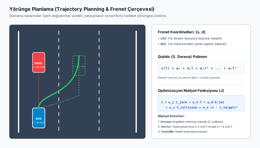
• $d(t)$ (lateral): Lateral offset perpendicular to the centerline. “Stay in lane” is now simply $d \approx 0$, and “change lanes left” is a simple ramp function $d: 0 \to +3.5\ \text{m}$.

CRITICAL — This is the real payoff of the Frenet Frame: longitudinal speed-profile planning and lateral in-lane/lane-change planning are decoupled into two independent one-dimensional optimization problems (formalized by Werling et al. 2010). Without this decoupling, every candidate trajectory would have to be optimized directly in the curved $[x,y]$ space — a far more computationally expensive proposition.

---

6. Jerk Minimization and Quintic Polynomials

FACT — Passengers generally don’t find acceleration (the sensation of speeding up/slowing down) uncomfortable even when it’s within safe limits; what actually feels unpleasant is jerk — the time derivative of acceleration:

$j(t) = \frac{da(t)}{dt} = \frac{d^3 s(t)}{dt^3}$

A sudden jerk (e.g. abruptly releasing the brake, sharply turning the wheel) is perceived as unsettling by the human inner ear and sense of balance even when physical acceleration limits are never exceeded. That’s why production planners optimize not just for “safe and legal” but explicitly for low-jerk, smooth trajectories. (The exact jerk threshold at which discomfort is felt is vehicle/passenger dependent; commonly cited practical upper bounds are on the order of $\sim 10\ \text{m/s}^3$ — [ASSUMPTION: the precise numeric value varies by manufacturer and comfort standard; only an order of magnitude is given here.])

The problem of minimizing a trajectory’s total jerk energy:

$\min \int_0^T j(t)^2\, dt \quad \text{s.t. boundary conditions on start/end position, velocity, acceleration}$

Via the calculus of variations, the analytical solution to this problem — when position, velocity, and acceleration are all specified at both $t=0$ and $t=T$ (a total of 6 boundary conditions) — turns out to be exactly a 5th-degree (quintic) polynomial:

$s(t) = a_0 + a_1 t + a_2 t^2 + a_3 t^3 + a_4 t^4 + a_5 t^5$

Boundary Condition	$t = 0$	$t = T$
Position	$s(0) = s_i$	$s(T) = s_f$
Velocity	$\dot s(0) = v_i$	$\dot s(T) = v_f$
Acceleration	$\ddot s(0) = a_i$	$\ddot s(T) = a_f$

These 6 equations form a linear system for the 6 unknown coefficients ($a_0 \ldots a_5$) and are solved directly. The same approach is applied independently to $d(t)$ (lateral motion) as well — the payoff of the Frenet decoupling kicks in again here.

EXAMPLE — In a lane-change maneuver, the lateral trajectory $d(t)$ starts at $t=0$ with $d_i = 0,\ \dot d_i = 0,\ \ddot d_i = 0$ (in the current lane, zero lateral velocity/acceleration) and ends at $t=T$ with $d_f = 3.5\ \text{m},\ \dot d_f = 0,\ \ddot d_f = 0$ (in the target lane, at rest again). The quintic polynomial satisfying these 6 conditions produces a smooth, S-shaped lateral transition with zero jerk at either endpoint.

---

7. Cost Function and Trajectory Selection

The motion planner doesn’t produce a single trajectory; in the Frenet lattice approach it samples tens to hundreds of candidate trajectories in $(s, d)$ space for different target durations and target positions, scores each one with a cost function, and selects the lowest-cost candidate:

$J = w_{jerk} J_{jerk} + w_{time} T + w_{collision} C + w_{lane} D_{lat} + w_{progress} P$

• $J_{jerk}$: total jerk energy along the trajectory (Section 6).
• $T$: time to complete the maneuver (too slow = low progress).
• $C$: collision risk penalty based on the minimum distance to dynamic obstacles.
• $D_{lat}$: penalty for deviating from the lane center.
• $P$: progress reward — how much closer the trajectory gets to the goal.

WARNING — Trajectories that carry collision risk (i.e., that intersect the predicted obstacle position within a given safety margin) are in practice assigned a cost of $J \to \infty$ — meaning these candidates are not given a “soft penalty” but are hard-eliminated from the candidate pool. The minimum-cost trajectory among the remaining candidates is selected and sent to the control layer (AD-11).

---

8. End-to-End Example: Changing Lanes to Pass a Slow Vehicle

The table below shows the concrete output each of the three layers produces for the same scenario (passing a truck traveling at $70\ \text{km/h}$ ahead on the highway):

Layer	Input	Decision/Output
Route	A→B route, current position	“Stay in lane 2 on this highway segment” (already decided at the route level, unchanged in this scenario)
Behavior	Ego speed $110\ \text{km/h}$, truck ahead at $70\ \text{km/h}$, $gap = 45\ \text{m}$ detected in the left lane	LANE_KEEP → PREPARE_LANE_CHANGE → EXECUTE_LANE_CHANGE (move left)
Motion	“Change lanes left” decision + truck’s predicted trajectory (AD-09)	Quintic-polynomial lateral trajectory $d: 0 \to 3.5\ \text{m}$ + a mild acceleration profile along $s(t)$, completing in $T \approx 4\ \text{s}$, jerk-optimal, collision-free concrete trajectory

This output chain ends with the motion planner’s trajectory being handed off to the control layer covered in AD-11 — the control layer converts this geometric trajectory into real steering angle and throttle/brake commands.

---

9. Notes from Real Systems

ASSUMPTION — The exact internal architecture of production autonomous driving stacks is generally not public; the notes below rely on publicly available technical talks and patents, and exact implementation details may vary by manufacturer and over time.

• Mobileye has published a mathematical framework called RSS (Responsibility-Sensitive Safety) to provide a safety guarantee at the behavior layer — it defines via formal rules which following distances/maneuvers count as “reasonably safe,” and bounds the behavior planner’s decision space with those rules.
• The Frenet-based sampling approach (Werling et al.) is widely used as the reference method for motion planning in academic literature and in many open-source autonomous driving stacks (e.g. Apollo, Autoware).
• Some newer-generation production stacks (e.g. Tesla’s recent FSD versions) have moved toward replacing part of the classical discrete FSM + optimization pipeline with end-to-end learned neural network components; the three-layer conceptual split remains a valid mental model in that case, but the boundary between layers may be blurrier in the actual software architecture (exact architectural details here are not fully public, hence marked ASSUMPTION).

---

Frequently Asked Questions (FAQ)

Q: What does a planner do when an obstacle suddenly appears in front of it?

FACT — In an emergency, the normal cost function weights are bypassed; an emergency braking or safety-corridor maneuver (Collision Avoidance Trajectory) is given top priority and is typically triggered by a separate, simpler, and more quickly verifiable “safety layer.”

Q: Why doesn’t the behavior planner directly produce a continuous trajectory?

Because a discrete decision space (stay in lane / change lanes / stop) is far more manageable for making verifiability and compliance with traffic rules auditable by humans; continuous optimization can then treat this discrete decision as given and operate in a much narrower search space.

Q: Does the Frenet frame have a downside?

Yes — if the road geometry has very sharp curve radii, or if the lane structure is ambiguous (e.g. inside an intersection, in a parking lot), defining the reference curve becomes difficult and the transform can lead to numerical instabilities; in these cases planners typically fall back to Cartesian-based methods.

---

Summary

• Planning is a three-layer hierarchy: Route (minutes, graph search) → Behavior (seconds, discrete decision process) → Motion (hundreds of ms, continuous trajectory).
• Route planning produces a lane-level graph path via A*/Dijkstra; behavior planning converts this into tactical maneuvers via an FSM or (PO)MDP; motion planning turns that maneuver into a physically executable trajectory.
• The Frenet $[s, d]$ system reduces road geometry’s complexity to two independent 1-dimensional problems, longitudinal and lateral.
• Human comfort is measured not by acceleration but by jerk; quintic polynomials with 6 boundary conditions are the jerk-optimal trajectory family.
• The cost function selects the safest, most comfortable, most progress-making candidate among the sampled trajectories; collision-risky candidates are hard-eliminated.

Sources and Verification Note

This lesson is based on Thrun et al. (Probabilistic Robotics), LaValle (Planning Algorithms), and Werling et al.’s academic work on optimal trajectory generation in the Frenet frame; the jerk-minimal quintic polynomial result is inspired by Flash & Hogan’s classic work on human arm movement and is widely reused in the robotics/autonomous driving literature. Details about the Mobileye RSS framework and the internal architecture of production stacks are based on publicly available technical publications and are marked ASSUMPTION above; the lastVerified date is the date of this lesson’s last technical review.

Next Lesson

• AD-11 — Vehicle Control: Lateral/Longitudinal Control and Trajectory Tracking: We’ll examine how the geometric trajectory produced in this lesson is converted into actual steering angle and throttle/brake commands, via control algorithms ranging from PID to Model Predictive Control (MPC).