
- Explain why prediction is necessary, and why planning (AD-10) needs to know not just where other agents ARE now but where they are LIKELY to be a few seconds ahead.
- Understand that future behavior is fundamentally uncertain and multi-modal, and that good prediction outputs a probability distribution rather than a single deterministic trajectory.
- Analyze the hierarchical relationship between intent estimation (coarse, behavioral) and trajectory forecasting (fine, geometric, uncertainty-bounded).
- Evaluate how kinematic history, map/lane topology, and social interaction context feed both intent and trajectory forecasting.
- Understand why modern learned prediction models are preferred over hand-coded rules, trained on large real-world driving datasets.
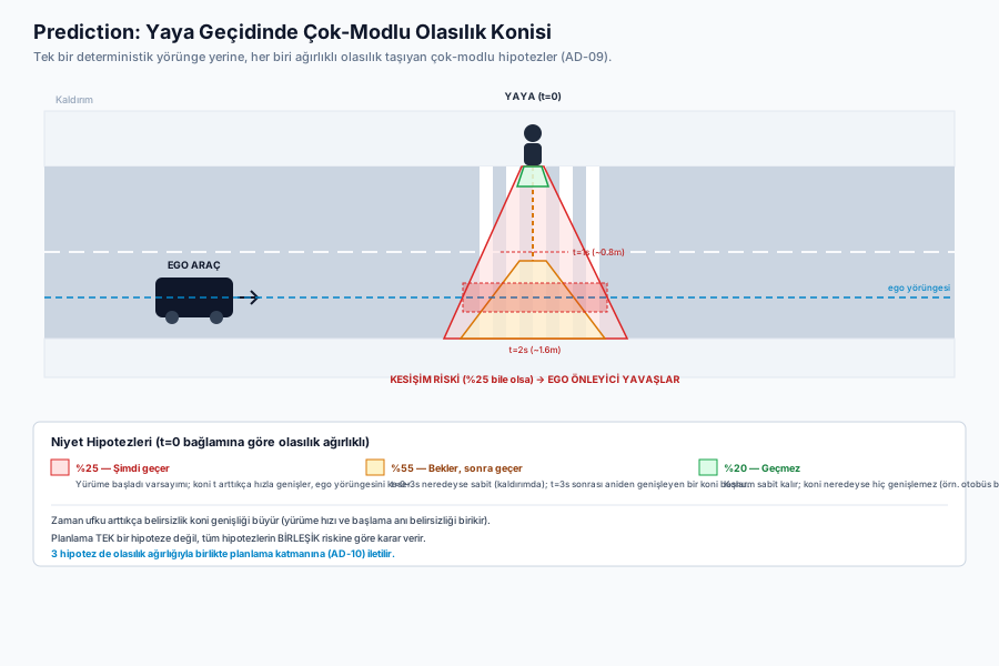
- Apply trajectory forecasting concretely through a worked example: a probability cone for a pedestrian at a crosswalk edge.
AD-09 — Prediction: Intent Estimation and Probabilistic Trajectory Forecasting
FACT — In AD-08 we covered the localization layers that let a vehicle know its OWN position to centimeter precision. But knowing where the vehicle itself is isn’t enough for safe driving on its own — it also needs to know where the OTHER agents around it (vehicles, pedestrians, cyclists) are likely to be a few seconds from now. This lesson covers the Prediction module that answers exactly that question.
In this lesson, we cover:
- Why Prediction? — What Planning Needs
- The Core Difficulty: The Future Is Uncertain and Multi-Modal
- The Hierarchy: From Intent Estimation to Trajectory Forecasting
- Context and Cue Sources: Kinematic, Map, Social Interaction
- The Modern Approach: Learned Models Instead of Hand-Coded Rules
- Worked Example: A Probability Cone at a Crosswalk Edge
- Comparison Table: Prediction Approaches
- FAQ, Summary, and Sources
1. Why Prediction? — What Planning Needs
FACT — In AD-06 we saw that perception produces every surrounding object’s position, class, and velocity at the CURRENT instant (). But the planning layer (AD-10) must evaluate the consequences of a maneuver decision (e.g., “change lanes now” or “slow down”) several seconds INTO THE FUTURE — because braking distance, maneuver duration, and other agents’ reaction times all take time. If planning decided based solely on positions at , it could never see IN ADVANCE that the car ahead will change lanes in 2 seconds, or that a pedestrian approaching an intersection will keep walking — every response would be reactive, arriving only AFTER the fact, and already too late.
The Prediction module takes perception’s current-instant object list as input and produces, for every dynamic agent, a sequence of likely future positions over the next several seconds (typically seconds). It is the temporal forecasting layer that bridges perception and planning:
2. The Core Difficulty: The Future Is Uncertain and Multi-Modal
CRITICAL — What makes prediction hard is, before any algorithmic complexity, a PHYSICAL fact: future behavior is fundamentally UNCERTAIN and often MULTI-MODAL — meaning there isn’t one “most likely” future, but several QUALITATIVELY distinct plausible futures. Consider a pedestrian standing at the edge of a crosswalk: that pedestrian might cross now, might cross in 3 seconds (after waiting for a signal), or might not cross at all and just keep waiting. These three scenarios aren’t “close” to each other — there’s no smooth transition between them; they are qualitatively separate possible futures.
This is why a good prediction system should output not a single deterministic trajectory, but a probability distribution spanning multiple possible futures:
Drawing a single line and saying “the pedestrian will cross here” silently discards two out of three scenarios — and if the scenario that actually happens is one of those discarded two, the planning layer is caught off guard. This is why modern prediction systems produce multiple trajectory hypotheses, each carrying a probability weight (or a spatial probability heatmap).
3. The Hierarchy: From Intent Estimation to Trajectory Forecasting
In practice, the prediction problem is solved as a two-layer hierarchy — one coarse/behavioral, one fine/geometric:
A. Intent Estimation — The Coarse Layer
The question: “What is this agent doing, behaviorally?” The output is a discrete behavior class: is it changing lanes, turning, going straight, stopping? For example, for a vehicle approaching an intersection, intent estimation might produce:
| Intent | Probability |
|---|---|
| Go straight | |
| Turn right | |
| U-turn |
B. Trajectory Forecasting — The Fine Layer
The question: “If this intent is realized, what GEOMETRIC PATH does the agent follow, and how uncertain is that path?” For each intent hypothesis, a concrete trajectory is produced, accompanied by an uncertainty cone that grows over time — as the time horizon () extends, even conditional on that intent being realized, uncertainty grows about exactly where the agent will be (fine-grained variables like the driver’s brake/throttle timing or the exact maneuver speed remain unknown).
INTERPRETATION — This two-layer split isn’t arbitrary: intent estimation (discrete, few options) is computationally cheap and lets the system rule out large errors early (e.g., predicting “will turn right” when it actually turns left); trajectory forecasting (continuous, high-dimensional) then expands EACH of these discrete hypotheses into fine geometric trajectories separately. Using this intermediate layer instead of going straight from “raw observation” to “continuous trajectory” in one step narrows the model’s search space and improves interpretability (engineers can get a partial answer to “why did the model produce this trajectory” by first looking at which intent it selected).
4. Context and Cue Sources: Kinematic, Map, Social Interaction
Both intent estimation and trajectory forecasting draw on three main context/cue sources:
A. Kinematic History
The agent’s directly observable state over the last few seconds — velocity, acceleration, and (for vehicles) turn signal. Physics-based short-term models are derived directly from this:
- Constant Velocity (CV):
- Constant Acceleration (CA):
These models are a reasonable approximation over very short horizons (roughly seconds) because physical inertia dominates on short timescales — a vehicle cannot suddenly turn 90 degrees within 0.3 seconds. But as the horizon lengthens () they fall short, because no kinematic model can “know” that a vehicle will turn at an upcoming intersection or that a driver is about to hit the accelerator — that information isn’t encoded in kinematics; it lives in the context sources below.
B. Map Context
Lane topology is a powerful behavioral cue. For example, a vehicle sitting in a right-turn-only lane will, almost by definition of that lane’s geometry, turn right — this is purely map-derived information, independent of kinematic history (the direct use, in prediction, of the HD map lane topology we covered in AD-08). Similarly, knowing which lanes connect to which exits at an upcoming intersection substantially narrows the intent probability distribution.
C. Social / Interaction Context
Traffic agents do not move INDEPENDENTLY of each other — they influence one another. A vehicle’s lane-change decision depends on the speed/gap of other vehicles in the target lane; a pedestrian’s crossing decision depends on the speed of an approaching vehicle and whether it’s slowing down. This mutual influence shows that modeling a single agent in isolation isn’t enough — the whole scene must be modeled jointly.
5. The Modern Approach: Learned Models Instead of Hand-Coded Rules
FACT — It is theoretically possible to combine the three context sources from Section 4 (kinematic + map + social) with hand-coded rules (“IF in a right-turn lane AND signal is on AND speed is dropping THEN right-turn probability = 90%”), but the sheer combinatorial explosion of real traffic scenes and their subtle exceptions (a pedestrian may keep walking while looking at their phone; a driver may turn without signaling) quickly makes hand-coded rule sets unmanageable.
This is why modern prediction systems feed these context sources into learned models (Graph Neural Networks — GNNs, Transformer architectures) instead; these models are trained on large-scale real-world driving data, learning the intent/trajectory relationship from millions of observed real human behaviors — inference is drawn from data rather than hand-written rules. The model jointly processes map topology, agents’ past trajectories, and the spatial relationships between them (often weighting “who influences whom” via an attention mechanism) to produce a multi-modal trajectory distribution.
ASSUMPTION — The exact architecture names used in this field (specific transformer variants, specific GNN structures) and which exact model a given company runs in production are a fast-moving and largely non-public area; the general principle stated here — “learned models, not hand-coded rules” — reflects a solid industry consensus, but no specific architecture’s current production status is claimed.
6. Worked Example: A Probability Cone at a Crosswalk Edge
EXAMPLE — A vehicle is approaching a crosswalk. A pedestrian standing on the sidewalk at the edge of the crosswalk has been detected by perception (AD-06). What does the prediction module produce for this pedestrian?
Intent layer (context at t=0):
- The pedestrian’s torso is oriented toward the road, and head position is turned toward the approaching vehicle → a cue supporting “will cross.”
- The pedestrian’s leg/body velocity is still near zero → hasn’t stepped off yet.
- Resulting intent distribution: , , .
Trajectory layer (for each intent hypothesis):
- Under the “crosses now” hypothesis: a central trajectory where the pedestrian has moved into the road by and by , wrapped in a growing uncertainty cone (the cone’s width at is larger than at , because of uncertainty in walking speed and the exact moment of stepping off).
- Under the “waits, then crosses” hypothesis: position is nearly static on the sidewalk for , then a rapidly widening cone begins after .
- Under the “does not cross” hypothesis: position stays essentially constant throughout, and the cone barely widens at all.
All three hypotheses, with their probability weights, are passed to the planning layer. Planning (AD-10) decides based not on the single most likely hypothesis, but on the COMBINED risk profile across ALL hypotheses — for instance, even at only 25% probability, if the “crosses now” hypothesis’s cone intersects the vehicle’s own trajectory, the vehicle still brakes preemptively, because a 25% collision risk is unacceptably large.
This example gives the abstract “multi-modal distribution” idea from Section 2 a concrete, numerical form: instead of a single “the pedestrian will be at point X” prediction, three probability-weighted futures are carried forward together, each with its own growing uncertainty cone.
7. Comparison Table: Prediction Approaches
| Approach | Time Horizon | Input | Strength | Weakness |
|---|---|---|---|---|
| Physics-based (CV/CA/Bicycle) | Kinematic history only | Computationally cheap, reliable short-term | Cannot anticipate tactical maneuvers (turns, lane changes) | |
| Intent Estimation | Kinematic + map topology | Discrete, interpretable, relatively cheap to compute | Doesn’t provide geometric trajectory detail | |
| Learned Multi-Modal Model (GNN/Transformer) | Kinematic + map + social interaction | Richest context, multi-modal probability distribution | Computationally expensive, requires large training datasets |
FAQ
Q: Why isn’t the prediction horizon extended beyond 8 seconds?
FACT — Traffic is chaotic and interactive; every additional second adds a multiplicative combination of every agent’s possible decisions in between. Beyond 8 seconds, the probability distribution widens so much (an uncertainty explosion) that the resulting “prediction” carries essentially no useful information — the cone grows so large it covers nearly the entire road and provides no useful constraint for planning.
Q: What happens if intent estimation gets it wrong (e.g., the model misses a 4th option)?
INTERPRETATION — Well-designed systems guard against this risk in two ways: (1) the intent distribution always includes a low-probability “other/uncertain” catch-all category, and (2) the planning layer decides based not on just the single most likely hypothesis but on the COMBINED risk across all hypotheses (as in the Section 6 example, a low-probability but high-consequence hypothesis can still warrant a precaution). Still, no prediction system is perfect — this is one of the reasons the planning layer (AD-10) is designed with additional safety margins.
Q: Are physics-based models entirely unnecessary now that learned models are richer?
INTERPRETATION — No; physics-based models are generally kept as a very-low-latency, computationally cheap fallback layer — they provide a simple, reliable backstop especially for situations requiring immediate, short-term reaction (e.g., emergency braking). Learned models are layered on top as a richer but more expensive upper layer; the two are not mutually exclusive.
Summary
- Prediction is the bridging layer that converts perception’s “where is it now” output into the “where is it likely to be in a few seconds” information planning needs.
- Future behavior is fundamentally uncertain and multi-modal; good prediction outputs a probability distribution spanning multiple possible futures rather than a single trajectory.
- The hierarchy moves from coarse intent estimation (changing lanes? turning?) to fine trajectory forecasting (a geometric path with a growing uncertainty cone).
- Kinematic history, map/lane topology, and social interaction between agents are the three core context sources feeding both intent and trajectory forecasting.
- Modern systems feed these contexts into learned models (GNN/Transformer) trained on large real-world driving datasets, rather than hand-coded rules.
- The crosswalk pedestrian example gives the multi-modal probability cone idea a concrete, numerical form: even a low-probability, high-consequence hypothesis can change the planning decision.
Sources and Verification Note
The prediction framework in this lesson draws on: Thrun, Burgard & Fox — Probabilistic Robotics (probabilistic state estimation, Bayesian filtering foundations); Paden et al. — A Survey of Motion Planning and Control Techniques for Self-Driving Urban Vehicles (kinematic/physics-based short-term models, the prediction-planning interface); Salzmann et al. — Trajectron++ (an example of a learned, multi-modal, map- and social-context-aware trajectory forecasting architecture); LaValle — Planning Algorithms (foundations of decision-making under uncertainty). Specific company/model architecture claims (exactly which architecture a given manufacturer runs in production) may not be public and may change over time; these are therefore marked as ASSUMPTION.
Next Lesson
- AD-10 — Planning: Route, Behavior and Motion/Trajectory Planning: This lesson covered probabilistically forecasting WHERE other agents will be in the future — AD-10 covers how the vehicle plans its OWN future safely, taking these forecasts as input.
Technical Diagrams
Quiz
What is the primary function of the Prediction module in an automated driving stack?
Prediction forecasts dynamic actor positions over a forward temporal horizon.
Which models excel in near-term (0 - 1.5s) trajectory forecasting?
Near-term trajectories are heavily governed by physical momentum and kinematic constraints.
What is the architectural term for forecasting multiple plausible future outcomes (e.g. turning vs proceeding straight)?
Multi-modal distributions output discrete probability-weighted trajectory candidates.
Which spatial cue indicates an unsignaled cut-in maneuver from an adjacent vehicle?
Lateral velocity vectors toward the lane boundary indicate aggressive cut-in intent.
Why are prediction horizons typically bounded to 3-8 seconds rather than 15-20 seconds?
Long horizons exhibit rapid uncertainty divergence due to complex interactive human decisions.