AD-07 — Sensor Fusion: Early, Late and Deep Fusion Architectures

FACT — In AD-05 we saw how a camera can fail alone in sun glare, how radar can fail in multipath propagation, and how LiDAR can fail in heavy rain. In AD-06 we covered how each sensor’s perception pipeline independently produces 3D boxes, class labels, track IDs, and free space. This lesson asks the next question: at which processing stage should these independent outputs — or the raw data before they even become outputs — be combined? The answer is not a single architecture; it is three families, each sitting at a different point on the information-richness/cost/robustness trade-off.

In this lesson, we will cover:

1. Why Sensor Fusion? — The Complementarity Principle
2. Late Fusion: Merging Object Lists
3. Early Fusion: Joint Reasoning at the Raw Data Level
4. Calibration and Synchronization: Early Fusion’s Hidden Engineering Cost
5. Mid-Level / Deep (BEV) Fusion: The Modern Industry Standard
6. Sensor Pairs: Camera+Radar, Camera+LiDAR, GNSS+IMU
7. Comparison Table: Fusion Level × Information Richness × Cost × Robustness
8. FAQ, Summary and Sources

---

1. Why Sensor Fusion? — The Complementarity Principle

FACT — No single sensor is sufficient for automated driving. Cameras excel at angular resolution and semantic classification but cannot directly measure radial velocity and degrade in fog/darkness. Radar excels in fog, rain, and direct Doppler velocity but has weak angular resolution. LiDAR excels at dense 3D geometry but is costly and degrades in heavy precipitation (see AD-05).

The underlying logic of sensor fusion is statistical: when two measurements with independent noise sources are combined, the resulting estimate’s variance (uncertainty) is smaller than either individual measurement’s. The optimal weighted combination of two independent Gaussian measurements with variances $\sigma_1^2$, $\sigma_2^2$ is:

$\hat{x}_{fused} = \frac{\sigma_2^2}{\sigma_1^2 + \sigma_2^2} x_1 + \frac{\sigma_1^2}{\sigma_1^2 + \sigma_2^2} x_2, \qquad \frac{1}{\sigma_{fused}^2} = \frac{1}{\sigma_1^2} + \frac{1}{\sigma_2^2}$

This simple relation already shows why fusion works: $\sigma_{fused}^2$ is always smaller than $\min(\sigma_1^2, \sigma_2^2)$. The real question is at which processing layer this combination happens — and that defines the three main families of fusion architecture.

---

2. Late Fusion: Merging Object Lists

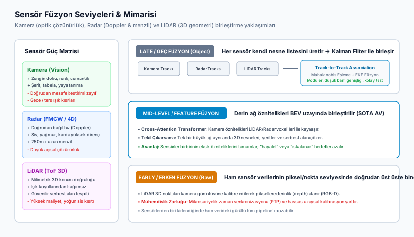
In Late (Object-Level) Fusion, each sensor modality runs its own independent perception pipeline end-to-end: the camera produces its own object list (2D/3D box + class), radar produces its own target list (range + Doppler velocity + weak class information), LiDAR produces its own 3D box list. Only these finished object lists are passed to a central fusion module.

Late Fusion Data Flow:

  Camera ──▶ [CNN Detector]   ──▶ Object List_cam ─┐
  Radar  ──▶ [CFAR + Tracker] ──▶ Object List_rad ─┼──▶ [Track-to-Track Association] ──▶ Unified World Model
  LiDAR  ──▶ [PointNet++ etc]──▶ Object List_lidar ─┘        (Association + EKF)

  Each sensor's own ECU / processing core runs independently.

The merge step consists of two sub-problems:

1. Association (Track-to-Track Matching): Which camera object and which radar target correspond to the “same physical vehicle”? This is typically solved with the Hungarian Algorithm over a cost matrix based on position, size, and temporal consistency.
2. Fusion: The state estimates of matched objects are reduced to a single tracked object via Extended Kalman Filtering (EKF) or Covariance Intersection (a conservative fusion method used when inter-sensor correlation is unknown).

FACT — Late fusion’s advantages: modularity (each sensor’s algorithm can be developed and tested independently; if one supplier’s stack changes, the others are unaffected), low bus load (sparse object lists, not raw data, are transmitted — CAN/Ethernet bandwidth is not a concern), and easy fault isolation (if one sensor pipeline fails, the others continue operating independently).

WARNING — Late fusion’s fundamental weakness is information loss. Each sensor discards candidates below its own detection confidence threshold in its own pipeline — and once discarded, no trace of them reaches the fusion stage. For example, if the camera does not report an ambiguous silhouette in fog as an “object” because it fell below threshold, even a clean radar Doppler return in that same region has nothing left to fuse against on the camera side — the two sensors’ raw uncertainties cannot complement each other, because the decision was already made independently, in isolation, by each one.

---

3. Early Fusion: Joint Reasoning at the Raw Data Level

In Early (Raw-Level) Fusion, no sensor makes a “decision” on its own. Raw or near-raw data — for example, a LiDAR 3D point cloud projected onto the camera’s pixel plane to form an RGB + depth matrix — is combined BEFORE the detection step, and a single model reasons over this unified representation.

Early Fusion Data Flow:

  LiDAR point cloud ──▶ [Calibrated projection: 3D → 2D pixel] ──┐
                                                                    ├──▶ [Joint RGB-D Input] ──▶ [Single Model] ──▶ Object List
  Camera pixel matrix ───────────────────────────────────────────┘

  Unlike late fusion, the decision point comes AFTER data is combined, in one pass.

The advantage is that it can catch objects that no single sensor would confidently detect alone: an object with weak contrast in the camera image but a sharp geometric boundary in LiDAR might fail both sensors’ individual detection thresholds separately, yet a joint model evaluating both cues together can detect it with confidence. Information loss is far smaller than in late fusion because no modality is “discarded” at an early stage.

The cost is precise calibration and synchronization requirements — the subject of the next section.

---

4. Calibration and Synchronization: Early Fusion’s Hidden Engineering Cost

For early fusion to work mathematically correctly, three distinct engineering problems must already be solved:

A. Extrinsic Calibration

Each sensor’s EXACT position ($x, y, z$) and orientation ($\phi, \theta, \psi$ — roll/pitch/yaw) relative to the vehicle body must be known. This yields the $4\times4$ homogeneous transformation matrix ($T = [R | t]$) that maps one sensor’s coordinate frame into another’s (e.g., LiDAR frame into camera frame):

$P_{camera} = T_{lidar}^{camera} \cdot P_{lidar}$

If this matrix is wrong by even a fraction of a millimeter/milliradian, a point seen by LiDAR projects onto the camera image a few pixels off from where it should be — this offset looks small for nearby objects, but at long range (>50m) a fraction-of-a-degree angular error translates into meters of positional error.

B. Intrinsic Calibration

Each sensor’s OWN internal parameters — for cameras, focal length, optical center, lens distortion coefficients (especially pronounced in fish-eye/wide-angle lenses); for LiDAR, laser channel angular offsets. Without correcting these, raw pixel coordinates cannot be converted to true angular direction.

C. Time Synchronization

CRITICAL — Different sensors have different frame rates (camera ~30-60 Hz, LiDAR ~10-20 Hz depending on rotation speed, radar ~15-20 Hz), and each one’s data capture instant (capture timestamp) differs at the microsecond level. If clocks are not aligned to a common reference, the position of a vehicle traveling at 100 km/h can shift by ~28 cm from a mere 10 ms timing offset between two sensors ($v \cdot \Delta t = 27.8 \text{ m/s} \times 0.01 \text{ s} \approx 0.28 \text{ m}$). In early fusion, this offset directly causes a mismatched RGB-D correspondence; in late fusion, it causes incorrect track-to-track association.

Industry solves this with hardware triggering (a “master” signal commands all sensors to capture simultaneously) and PTP (Precision Time Protocol, IEEE 1588 / the automotive IEEE 802.1AS variant): all ECUs are synchronized to a common network clock at microsecond precision, and every data packet is timestamped against this shared clock.

INTERPRETATION — This calibration/synchronization burden explains why “pure” early fusion is less common in practice than late fusion — most production systems instead gravitate toward the mid-level fusion described next, because a learned feature representation can be somewhat more tolerant of small calibration errors than raw pixel/point correspondence (the network can partially learn to compensate for minor alignment inconsistencies seen during training).

---

5. Mid-Level / Deep (BEV) Fusion: The Modern Industry Standard

Mid-level (feature-level) fusion sits between early and late fusion and is where most of today’s deep-learning-based perception stack R&D is concentrated. Each modality is passed not through raw data, nor all the way to a finished object list — but through its own partial neural network, producing an intermediate learned feature representation (feature space). The final decision is made by a joint downstream network operating in this shared feature space.

Mid-Level / BEV Fusion Data Flow:

  Camera ──▶ [Backbone CNN]      ──▶ Camera feature map ─┐
  Radar  ──▶ [Backbone]          ──▶ Radar feature tensor ─┼──▶ [Projection to BEV grid] ──▶ [Joint Head Network] ──▶ Object List
  LiDAR  ──▶ [Voxel/Backbone]    ──▶ LiDAR voxel features ─┘        (Cross-Attention / Transformer)

  The decision is made neither on raw data nor on a finished object list, but in an INTERMEDIATE feature layer.

In modern architectures this is frequently done via a shared BEV (Bird’s-Eye View) grid: each modality’s features are projected onto a fixed top-down grid around the vehicle (e.g., 0.5m × 0.5m cells), and a Transformer Cross-Attention network or convolutional head then jointly evaluates all modalities over this shared spatial grid to produce the final detections.

INTERPRETATION — BEV feature fusion’s rapid industry adoption stems from the fact that it approaches early fusion’s information richness while being able to partially “smooth over” calibration/synchronization sensitivity through learned weights — the network learns to compensate to some degree for small alignment inconsistencies it sees in training data. This does not fully preserve late fusion’s modularity, nor does it carry early fusion’s fragility; much of today’s new L3/L4 perception stack R&D — from Tesla’s camera-centric BEV approach to many LiDAR-centric L4 companies’ BEV-transformer architectures — is understood to be concentrated here.

---

6. Sensor Pairs: Camera+Radar, Camera+LiDAR, GNSS+IMU

A. Camera + Radar (The Backbone of Production ADAS)

The camera reports WHAT an object is (class: vehicle/pedestrian/cyclist) and its lateral bounds (high angular resolution); radar provides exact range and instantaneous relative velocity (measured directly via Doppler, not derived). These complement each other because a camera cannot directly measure radial velocity (only a coarse estimate via optical flow across successive frames), while radar cannot reliably classify object type.

B. Camera + LiDAR (High-Level Autonomy, L3/L4)

LiDAR draws the precise 3D box and range; the camera supplies traffic light color, sign text, and fine-grained class distinctions (e.g., bus vs. truck). In early fusion, LiDAR points can be projected onto camera pixels to form an RGB-D matrix (see Section 3); in mid-level fusion, the two merge within separate BEV feature layers.

C. GNSS + IMU (Localization Fusion — the Foundation of AD-08)

• Loose Coupling: The $(x,y,z)$ position solution the GNSS receiver has ALREADY computed internally is combined with the IMU integration output in an outer Kalman filter. Simple, but fragile against GNSS’s own internal failure modes (e.g., the GNSS solution suddenly degrading when satellite count drops).
• Tight Coupling: The GNSS receiver’s NOT-YET-resolved raw measurements — pseudorange and carrier phase — are fused directly with IMU acceleration/angular rate data into a SINGLE EKF state vector. Even if satellite count drops below 4 (the minimum required for a 3D position fix), the partial information from remaining satellites can still correct the IMU estimate — this is impossible in loose coupling, because the GNSS receiver would simply report “no fix” and provide nothing at all.

This distinction is the direct localization-domain reflection of the general late-fusion (loose coupling uses the finished GNSS solution) vs. early/tight-fusion (uses raw pseudorange) principle — we will deepen this in AD-08 in the context of GNSS-RTK and dead reckoning.

---

7. Comparison Table

Fusion Level	Information Richness	Computational Cost	Calibration Sensitivity	Failure-Mode Robustness	Typical Use
Late (Object-Level)	Low — each sensor discards below its own threshold	Low — sparse object lists transmitted	Loose — coarse position/time agreement suffices	High — one sensor’s failure leaves others operating independently	Production L2 ADAS, cost-constrained systems
Mid-Level/BEV (Feature-Level)	High — learned representation, partial tolerance	High — large neural networks, needs GPU/NPU	Moderate — network can partially compensate for small errors	Moderate — a shared head network can be affected if one modality degrades	Modern L3/L4 perception stacks (BEV-Transformer)
Early (Raw-Level)	Highest — no modality discarded early	Moderate-High — but single-pass, no redundant processing	Very tight — pixel/point-level alignment required	Low — calibration/sync errors corrupt the entire pipeline	Research systems, dedicated RGB-D hardware platforms

---

FAQ

Q: Does a failed or dirty sensor break the whole fusion pipeline?

FACT — In a well-designed fusion architecture, every sensor output carries a confidence score (covariance/confidence). When a sensor is degraded (e.g., mud on the camera lens, ice on the radar antenna), that modality’s covariance is inflated; the Kalman filter or feature-weighting mechanism dynamically pushes that sensor’s influence toward zero. No sensor is ever used “blindly.”

Q: Does early fusion always produce the most accurate result?

INTERPRETATION — In theory, yes, since information loss is minimized — but in practice, calibration/synchronization errors can irrecoverably corrupt the entire result in early fusion, whereas in late fusion a faulty sensor can remain isolated. So “which architecture is most accurate” depends on hardware quality, compute budget, and safety requirements — there is no single universal answer.

Q: Will mid-level BEV fusion fully replace late fusion?

ASSUMPTION — The industry trend appears to lean strongly this way, especially on new L3/L4 platforms, but low-cost production L2 systems still benefit from late fusion’s modularity/cost advantage, so a gradual shift rather than a complete replacement is expected. This is a forecast that may change with individual company strategies.

---

Summary

• Sensor fusion combines measurements with independent noise sources to produce a lower-variance world model than any single sensor alone.
• Late fusion (object-list level) is modular and low-cost, but candidates discarded early never reach fusion at all.
• Early fusion (raw-data level) carries the richest information but requires precise extrinsic/intrinsic calibration and microsecond-level time synchronization (PTP).
• Mid-level/BEV feature fusion is the middle path modern deep learning stacks focus on: rich information plus partial calibration tolerance.
• Camera+radar, camera+LiDAR, and GNSS+IMU pairs are concrete industry applications of the complementarity principle; GNSS+IMU’s loose/tight coupling distinction directly mirrors the late/early fusion principle in the localization domain.

Sources and Verification Note

The fusion taxonomy and mathematical framework in this lesson draw on: Thrun, Burgard & Fox — Probabilistic Robotics (Bayes filtering and Kalman fusion fundamentals); Bar-Shalom, Li & Kirubarajan — Estimation with Applications to Tracking and Navigation (track-to-track association, covariance intersection); Szeliski — Computer Vision: Algorithms and Applications (camera calibration, projection geometry); Chen et al. — MV3D (an example early/mid-level multi-modal fusion architecture). The time synchronization and PTP section rests on the general principles of IEEE 1588 / IEEE 802.1AS; company-specific architecture details (e.g., which manufacturer uses exactly which fusion level) are based on publicly available technical presentations and can change over time, hence flagged as ASSUMPTION.

Next Lesson

• AD-08 — Localization: GNSS/RTK, Dead Reckoning, HD Maps and SLAM: This lesson covered the loose/tight coupling distinction in GNSS+IMU fusion — AD-08 builds on this foundation with GNSS-RTK centimeter-level correction, IMU drift dynamics, HD map registration, and SLAM.