
- Define the 4 core outputs of the perception layer (3D bounding box, class label, track ID, free space) and explain why the planning layer needs each of them.
- Explain the transition from classical feature-based object detection (HOG+SVM) to modern deep-learning (CNN-based) architectures, and the transition from 2D pixels to 3D metric space (BEV).
- Derive the data-association problem in Multi-Object Tracking (MOT), the Kalman Filter equations, and Hungarian Algorithm matching.
- Understand why free-space segmentation is conceptually different from and complementary to discrete object detection, and the role of Occupancy Grid mapping in collision safety.
- Understand why perception-level (early/mid) fusion outperforms fusion at the object-list level alone.
AD-06 — Perception: Object Detection, Classification, Tracking and Free Space
FACT — Each of the camera, radar, and LiDAR modalities covered in AD-04 and AD-05 produces raw data streams that are limited by their own physical principle, partially degraded, and repeating tens of times per second. The job of the Perception layer is to convert this heterogeneous, noisy raw data into a clean, structured, temporally consistent World Model that the planning and decision layers can consume directly. This is the most computationally intensive layer in the autonomous driving software stack.
In this lesson, you will learn:
- The 4 Outputs of the Perception Layer — 3D box, class, track, free space.
- Object Detection: From Classical to Deep Learning — from HOG+SVM to CNN-based detectors, from 2D to 3D/BEV.
- Classification — semantic labeling and confidence scores.
- Multi-Object Tracking (MOT) — Kalman Filter, data association, the Hungarian Algorithm.
- Free Space and Occupancy Grid — the complement to discrete object detection.
- Perception-Level Fusion — a preview of early/late fusion (a bridge to AD-07).
- Worked Example — the perception output for a busy urban intersection frame.
1. The Perception Layer’s Job and Its 4 Core Outputs
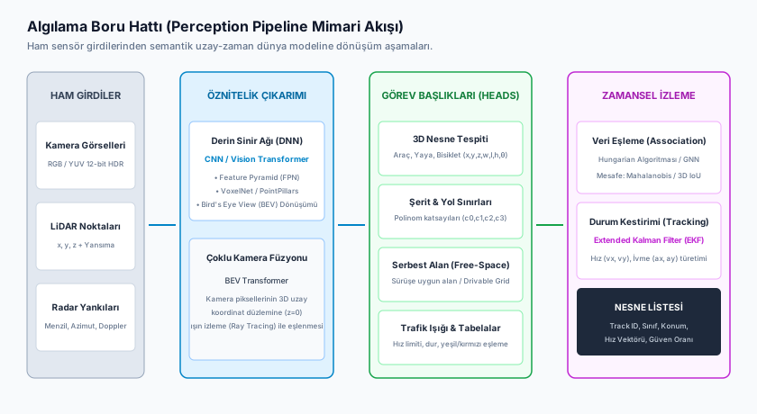
FACT — The perception layer’s output consists of 4 numerically well-defined components that can be consumed directly as input to the planning layer:
- 3D Bounding Boxes: For each detected object, metric-space coordinates — center position, dimensions (width/length/height), and yaw angle (orientation).
- Semantic Classification: Vehicle (car, truck, bus), Vulnerable Road User — VRU (pedestrian, cyclist, motorcyclist), static obstacle, or animal; each class comes with a confidence score.
- Temporal Tracking (Track ID & Velocity): A persistent identifier (Track ID) assigned to each object, plus derived instantaneous velocity/acceleration vectors .
- Road Structure and Free Space: Lane-marking polynomials, road boundaries, and a drivable free-space grid map.
These four outputs aren’t independent of each other — the track ID and velocity vector are derived from associating 3D boxes across consecutive frames (§4); the free-space map, by contrast, is an entirely different representation from the discrete object list (§5). The planning layer (covered in later lessons) consumes both simultaneously: “avoid this object” (discrete list) and “you can drive in this region” (continuous area).
2. Object Detection: From Classical to Deep Learning
2.1 The Classical Computer Vision Approach
Pre-2012 automotive vision systems relied on hand-crafted feature extractors. One of the most common examples is the HOG (Histogram of Oriented Gradients) + SVM (Support Vector Machine) pipeline: the image is divided into small cells, an edge-orientation histogram is computed for each cell, and this feature vector is fed to a pre-trained SVM classifier. This approach is computationally cheap and can run in real time on embedded hardware, but it has a fundamental weakness: the features are designed by humans — assumptions about which edge pattern constitutes a “pedestrian” are baked into the code. A change in lighting, partial occlusion, or an unusual pose (e.g., a bent-over pedestrian) can invalidate these assumptions, and detection fails.
2.2 The Deep Learning Revolution: End-to-End Learned Features
INTERPRETATION — Starting in 2012, convolutional neural networks (CNNs) made feature extraction learnable from data instead of hand-designed. A CNN-based detector (two-stage, region-proposal-based architectures like Faster R-CNN, or single-stage, anchor-based architectures like YOLO/SSD), trained on millions of labeled images, learns the concept of “pedestrian” implicitly across thousands of variations (different poses, lighting, partial occlusion). This removes the hand-coded assumption ceiling of the classical approach — at the cost of requiring far more compute (GPU/NPU) and very large, carefully labeled datasets.
Modern detectors fall into two families: two-stage (region proposals — “there might be an object here” — are generated first, then each region is classified; more accurate, slower) and single-stage (region proposal and classification are combined in a single network pass; faster, better suited to production ADAS’s real-time requirements). The standard metric for measuring detection quality is IoU (Intersection over Union):
Here is the predicted box and is the ground-truth box. A detection is counted as “correct” once IoU exceeds a given threshold (typically 0.5-0.7); this metric is used both during training and in the data-association step in §4.
2.3 From 2D to 3D: Camera Geometry and the BEV Transform
Classical 2D object detection stays in the pixel plane — but for a vehicle to brake, it needs to know how many meters away an object is (metric 3D space). Pixel coordinates are transformed into 3D rays using the camera’s intrinsic matrix (focal length and optical center ) and extrinsic matrix (the camera’s position/orientation relative to the vehicle body); combined with LiDAR/stereo depth information, the actual 3D point along this ray is resolved.
Modern architectures (such as BEVDet, BEVFormer) perform this transformation not object by object, but for the entire scene at once: the image feature maps from multiple cameras are projected directly into a top-down (Bird’s Eye View — BEV) plane using spatial cross-attention mechanisms. The advantage of the BEV representation is that it makes it natural to combine the output of different cameras (and even radar/LiDAR) in a shared metric coordinate system — which is the technical foundation for the perception-level fusion we’ll cover in §6.
3. Classification: Semantic Labeling
Each detected bounding box is passed through a classification head and mapped to a class label and a confidence score. The network’s output layer typically produces a probability for each candidate class via a softmax function:
Here is the network’s raw output (logit) for class , and is the total number of classes. The highest-probability class is assigned as the final label, but the probability value itself (the confidence score) is also passed to the planning layer — a low-confidence detection (e.g., “55% pedestrian, 40% cyclist”) can trigger a more conservative response on the planning side (e.g., earlier deceleration).
WARNING — When the classifier encounters an object not represented in the training dataset (out-of-distribution — OOD), it cannot produce a reliable result: an overturned refrigerator on the road, or an unusual load, might not clearly match any trained class. This is exactly why the Occupancy Grid approach in §5 exists — a safety net that is independent of classification.
4. Multi-Object Tracking (MOT)
FACT — Detecting objects independently in every frame isn’t enough; the system must know that a detection in the previous frame and a detection in the current frame are the same physical object (data association), and derive velocity/acceleration from that relationship. This consists of two sub-problems: state estimation and data association.
4.1 State Estimation: The Kalman Filter
An object’s state (position + velocity) is classically tracked with a Kalman Filter — an optimal, computationally cheap recursive estimator for linear systems with Gaussian noise. It consists of two steps:
Prediction: The previous state is propagated to the next time step using a physical motion model (typically constant velocity, or constant acceleration):
Here is the state vector (position, velocity), is the motion model matrix, is the state covariance (uncertainty), and is process noise.
Update: When a new sensor measurement () arrives, the state is updated by weighting the difference between the prediction and the measurement (the innovation) with the Kalman gain ():
Here is the measurement matrix and is the measurement noise covariance. The Kalman gain weights the measurement more heavily if it’s more trustworthy (low ), and the prediction more heavily if it’s more trustworthy — this is the statistically optimal way to combine two uncertain sources of information.
4.2 Data Association: The Hungarian Algorithm
If a frame has existing tracks and new detections, which track matches which detection is not known in advance — this is the data association problem. A cost (similarity) is computed for every track-detection pair, typically using one of two metrics:
- 3D IoU: The generalization of the IoU formula from §2.2 to 3D boxes.
- Mahalanobis Distance: A statistical distance that accounts for the Kalman filter’s state uncertainty:
Here is the innovation covariance. Unlike Euclidean distance, this allows a wider matching “tolerance” for a track with higher uncertainty.
Given the resulting cost matrix, the Hungarian Algorithm solves the globally optimal assignment that minimizes total cost in polynomial time () — guaranteeing the correct result even in cases where a greedy match (matching each track to its nearest detection in sequence) could get stuck in a locally optimal but wrong assignment.
CRITICAL — An unmatched detection starts a new track (an object newly entering the scene); an unmatched track is marked as “lost” (coasting) for a few frames and kept alive only via the prediction step (without a measurement) — if no match arrives for a set number of frames, the track is deleted. This mechanism ensures an object doesn’t lose its track ID during a brief occlusion (AD-05 §1.4).
5. Free Space and Occupancy Grid
EXAMPLE — An overturned refrigerator on the road, or spilled cargo, may have no clear match in any classifier’s training set (an out-of-distribution object, per the warning in §3). An autonomous vehicle must not hit it, even if it can’t identify it as a “vehicle” or a “pedestrian.”
This is why free-space / drivable-area estimation is conceptually different from discrete object detection: object detection says “there is a known object of class X here,” while free-space estimation answers the question “is this region safe to drive through,” without needing any discrete object classification at all. This is typically done through semantic segmentation of the road surface — every pixel/cell is assigned a class such as “drivable road,” “curb,” “construction barrier,” or “other vehicle”; unlike bounding boxes, segmentation is a continuous spatial representation, and it also covers structures — like intersection edges or construction delineator cones — that aren’t a discrete “object” but still directly affect planning.
The Occupancy Grid takes this idea into a probabilistic framework:
- The area around the vehicle is divided into cells, typically .
- LiDAR point cloud and stereo depth rays assign an occupancy probability to each cell.
- Cells whose probability exceeds a given threshold are declared “no-drive zones” — even without knowing what the object is.
INTERPRETATION — The Occupancy Grid is a safety net that kicks in even when classification fails: even if the object detection + classification pipeline incorrectly decides “this is an OOD object, safe to ignore,” the high occupancy probability in the same region independently signals to the planning layer “do not pass through here.” The two representations (discrete object list + continuous occupancy grid) work together — neither replaces the other.
6. Perception-Level Fusion: Why Not Just at the Object-List Level
INTERPRETATION — It’s worth previewing here the three levels of sensor fusion we’ll cover in full in AD-07, because modern perception architecture is directly shaped by this choice:
- Late (Object-Level) Fusion: Each sensor independently produces its own object list (the camera its detections, the radar its detections), and these lists are merged afterward. Simple and modular, but has a limit.
- Early/Mid (Feature-Level) Fusion: Raw or intermediate-layer feature maps (e.g., the BEV feature maps in §2.3) are combined into a shared representation before object detection is finalized.
Why does this distinction matter? Because in late fusion, if, say, a radar return is sub-threshold weak (filtered out by a low confidence score) and, at the same time, a camera detection is also sub-threshold weak due to partial occlusion, both sensors report that object as “absent” — there is nothing left to combine. In early/mid fusion, these two separately weak signals can instead be pooled in a shared feature space before object detection is finalized, and the combined signal can cross the threshold to produce a valid detection. This is why modern production architectures (especially BEV-based networks) are increasingly moving toward combining sensor data at the feature level rather than only at the final object-list level — which is exactly the subject of AD-07.
7. Worked Example: A Busy Urban Intersection Frame
EXAMPLE — The table below shows a typical output produced by a camera + LiDAR + radar fusion perception pipeline for a single frame (simplified, for conceptual purposes):
| Track ID | Class (confidence) | Position [m, ego-relative] | Velocity [m/s] | Uncertainty () |
|---|---|---|---|---|
| 1042 | Pedestrian (0.94) | (3.2, 8.1) | (0.0, -1.1) | Low |
| 1043 | Cyclist (0.81) | (-2.5, 15.0) | (2.8, 0.3) | Medium |
| 1044 | Car (0.97) | (1.0, 32.4) | (-0.5, 8.9) | Low |
| 1046 | Vehicle (0.62) — partial occlusion | (18.0, 40.0) | (0.1, 7.5) | High (coasting, 2 frames) |
| — | Unknown (OOD) | Occupancy grid: cell (5,5) at | — | No class, occupancy only |
Alongside this, a drivable-area mask is generated for the scene: the central portion of the intersection and the opposing lane are marked “drivable,” while the curb/sidewalk strip and the cells around track 1046 (expanded with an uncertainty margin due to partial visibility) are marked “no-drive.”
INTERPRETATION — This single frame embodies everything covered in this lesson: tracks 1042 and 1044 are tracked with high confidence, while 1046 is still tracked via the §4.1 “coasting” mechanism (a brief occlusion, AD-05 §1.4) but flagged with high uncertainty; a region that cannot be classified is passed to planning not as a separate object, but directly as “area to avoid,” thanks to the independent safety net of the occupancy grid in §5.
Frequently Asked Questions (FAQ)
Q: Why can’t a camera measure 3D distance as precisely as LiDAR?
FACT — A camera projects the 3D world onto a 2D plane (perspective projection); depth information is physically lost during this projection and, as explained in §2.3, must be estimated by AI. LiDAR, as we saw in AD-04 §4, directly measures the round-trip time of flight of a photon, so it delivers distance at millimeter precision, based on measurement rather than estimation.
Q: Why can the Kalman Filter fall short for non-linear motion models (e.g., a vehicle taking a sharp turn)?
WARNING — The standard Kalman Filter assumes a linear system; under non-linear dynamics like a sharp turn, the state-transition model is no longer linear. Production systems typically switch to non-linear variants such as the Extended Kalman Filter (EKF) or Unscented Kalman Filter (UKF) in this case (the same family of EKF we saw applied to GNSS-IMU fusion in AD-04 §6.3).
Q: If we have an Occupancy Grid, why do we still need a separate object classification layer?
INTERPRETATION — The occupancy grid only says “something is/isn’t here” — it carries no velocity or intent information. Predicting whether a pedestrian is about to enter the intersection requires class information (VRU or vehicle?) and track history (velocity/acceleration trend) — the two (occupancy + object list) complement each other; neither replaces the other.
Summary
- Perception is the most computationally intensive layer, converting raw heterogeneous sensor input into 3D bounding boxes, class labels, persistent tracks, and free space.
- Classical feature-based detection (HOG+SVM) is limited by hand-designed assumptions, while deep-learning CNN detectors learn features end-to-end from data; IoU is the standard accuracy metric.
- BEV architecture uses camera intrinsic/extrinsic geometry to combine multi-camera (and multi-sensor) data into a shared top-down metric plane.
- MOT consists of two sub-problems: state estimation via the Kalman Filter (prediction + update) and globally optimal data association via the Hungarian Algorithm (using IoU or Mahalanobis distance).
- The Occupancy Grid is a safety net, independent of classification, against unclassifiable (OOD) objects; free-space segmentation complements discrete object detection rather than replacing it.
- Modern architectures are increasingly moving from late (object-list) fusion toward early/mid (feature-level) fusion — because separately sub-threshold weak signals can combine into a valid detection in a shared feature space (the subject of AD-07).
Sources and Verification Note
The mathematical framework presented in this lesson (the Kalman Filter, data association) is based on the classical tracking literature of Thrun et al. (Probabilistic Robotics) and Bar-Shalom, Li & Kirubarajan (Estimation with Applications to Tracking and Navigation); camera geometry and the BEV transform are based on Szeliski’s foundational work (Computer Vision: Algorithms and Applications). References to specific modern deep-learning architectures (such as BEVDet, BEVFormer) are for conceptual reference and should be treated as ASSUMPTION, since architectural details evolve rapidly — current architecture comparisons should be verified against the relevant academic literature.
Next Lesson
- AD-07 — Sensor Fusion: Early, Late, and Mid-Level Fusion Architectures: We’ll cover the early/late/mid fusion taxonomy previewed in this lesson in full — combining AD-05’s complementary sensor weaknesses with AD-06’s perception architecture to examine the real fusion architectures used in production systems (camera-radar early fusion, LiDAR-camera mid fusion).
Technical Diagrams
Quiz
What parameters define a 3D bounding box generated by a perception module?
A 3D bounding box parameterizes metric translation, scale, and spatial orientation.
What is the primary architectural advantage of Bird's Eye View (BEV) perception?
BEV representations eliminate perspective distortion, presenting planning modules with metric Cartesian features.
What is the core function of a Kalman Filter within a Multi-Object Tracking (MOT) pipeline?
Kalman filtering balances kinematic process prediction against noisy measurement uncertainty.
How does an autonomous vehicle avoid unclassified, out-of-distribution road hazards (e.g. fallen cargo)?
Occupancy grids map physical volumetric occupancy, preventing collisions with unknown obstacles.
Which combinatorial optimization algorithm matches incoming sensor detections with existing tracks?
The Hungarian algorithm resolves bipartite assignment between tracks and detections based on cost matrices.
Glossary
| English Term | Definition |
|---|---|
| LiDAR (Light Detection and Ranging) | An optical sensor emitting pulsed eye-safe laser beams (905 nm or 1550 nm) that measures time-of-flight to generate dense, accurate 3D spatial point clouds. |
| Bird's Eye View (BEV) | A unified, top-down metric Cartesian spatial representation where perspective camera feeds, radar, and lidar data are transformed to enable multi-task perception and planning. |
| Object and Event Detection and Response (OEDR) | The task of detecting and responding appropriately to objects and events in the driving environment (e.g. noticing the vehicle ahead is braking and applying one's own brakes accordingly). One of the three components of the Dynamic Driving Task (DDT). |