
- Explain the physical principles behind the 6 core modalities that make up the ADAS sensor suite.
- Derive how a single FMCW radar chirp resolves both range and Doppler relative velocity simultaneously at 77–81 GHz.
- Evaluate mechanical, solid-state (MEMS), and flash LiDAR architectures, and the 905 nm/1550 nm power-range trade-off through the physics of eye safety.
- Understand the camera FOV/resolution trade-off and the logic behind a multi-focal (trifocal) camera cluster.
- Understand the foundations of centimeter-level positioning through GNSS-RTK and 6-axis IMU integration, and why it is necessary.
AD-04 — ADAS Sensors: Camera, Radar, LiDAR, Ultrasonic, GNSS and IMU
FACT — An autonomous vehicle has a perceptual set no human driver has ever had: it simultaneously processes visible light, millimeter-wave radio frequency, infrared laser pulses, acoustic pressure waves, and satellite timing signals. This lesson lays the foundation for the hardware-level operating principles of those five physical modalities (plus their complement, the IMU), their relative strengths and weaknesses, and why no single one is ever sufficient on its own.
In this lesson, you will learn:
- The Electromagnetic Spectrum and Sensor Modalities — which wavelength does which job.
- Automotive Cameras — mono/stereo, rolling/global shutter, HDR, multi-focal camera clusters.
- 77–81 GHz FMCW Radar — resolving range and velocity in a single chirp, why it works in any weather, 4D imaging radar.
- LiDAR Architectures — mechanical, solid-state (MEMS), flash; the 905 nm vs. 1550 nm eye-safety physics.
- Ultrasonic Sensors — why they are still indispensable.
- GNSS-RTK + IMU Fusion — the foundation of centimeter-level positioning.
- Case Study: Sensor Suite Philosophies — Tesla Vision, Waymo, Mercedes/BMW L3.
1. The Electromagnetic Spectrum and Sensor Modalities
FACT — Autonomous vehicles cannot depend on a single sensor, because how each physical wavelength interacts with matter (reflection, scattering, absorption) differs fundamentally. This physical diversity is also the root of the “every sensor has a blind spot” principle we’ll cover in AD-05.
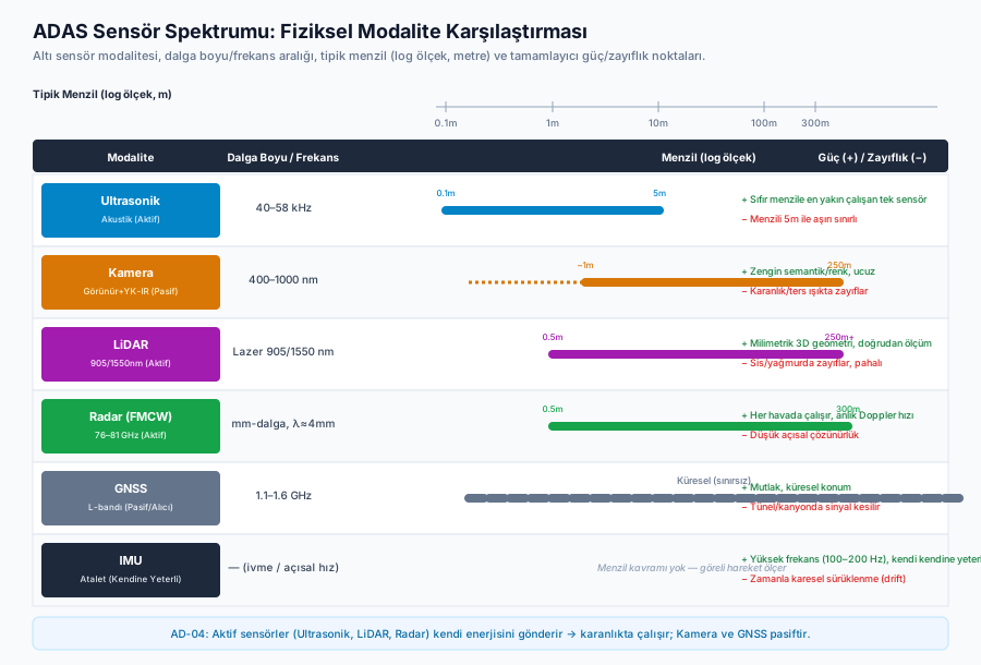
| Modality | Wavelength / Frequency | Typical Range | Directly Measures | Active/Passive |
|---|---|---|---|---|
| Ultrasonic | Acoustic, 40–58 kHz | 0.1 – 5 m | Distance (ToF) | Active |
| Camera | Visible + near-IR, 400–1000 nm | 0 – 250 m | Light intensity / color | Passive |
| LiDAR | Laser, 905 nm or 1550 nm | 0.5 – 250 m+ | Distance (ToF), intensity | Active |
| Radar | Millimeter wave, 76–81 GHz (λ ≈ 4 mm) | 0.5 – 300 m | Distance + relative velocity | Active |
| GNSS | L-band, 1.1–1.6 GHz | Global | Absolute position | Passive (receiver) |
| IMU | — (inertial) | — | Acceleration, angular velocity | Self-sufficient |
The “Active/Passive” distinction in this table has a critical engineering consequence: active sensors (radar, LiDAR, ultrasonic) emit their own energy into the environment and measure its reflection, so they can operate in complete darkness; passive sensors (camera) depend entirely on ambient photons already present in the scene.
2. Automotive Cameras (Vision Sensors)
2.1 Mono vs. Stereo
A single (mono) camera cannot measure depth directly; it estimates 3D distance from an object’s apparent size and learned visual cues (perspective, occlusion, size priors) via a neural network. A stereo camera pair, by contrast, produces genuine metric depth through classical triangulation:
Here is the focal length, is the baseline between the two cameras, and is the disparity (the pixel shift of the same object between the two images). A larger baseline improves depth accuracy at longer distances — but the baseline that can physically fit within a vehicle body is limited (typically 12–20 cm), which caps the practical depth range of stereo cameras at highway distances (150 m+).
2.2 Rolling Shutter vs. Global Shutter
WARNING — A CMOS sensor with a rolling shutter reads each row of the image sequentially (top to bottom) with a millisecond-scale delay between rows. In a static scene this is invisible; but an object moving at high relative velocity with respect to the sensor (for example, an oncoming vehicle closing at relative speed, or a spinning wheel) is “captured” at a slightly different instant on each row. The result: vertical objects appear skewed, rotating objects appear distorted (the “jello effect”) — this causes bounding-box corners to be misplaced and produces tracking errors.
With a global shutter, the entire pixel array is sampled at the same instant (a single timestamp), which eliminates this geometric distortion entirely. The cost: because global shutter sensors require extra per-pixel storage circuitry, they have lower light sensitivity (fill factor) than rolling shutter sensors and are generally more expensive. This is why production ADAS systems prefer global shutter for stereo pairs and front-facing cameras that require high speed/high precision, while the cost advantage of rolling shutter remains acceptable for low-speed/parking cameras.
2.3 HDR: Why 120–140 dB Is Needed
The human eye’s instantaneous dynamic range is roughly 10–14 stops (about 60–90 dB), while a standard CMOS sensor captures only ~60–70 dB in a single exposure. But a tunnel-exit scene can contain both a shaded tunnel interior (a few lux) and direct sunlight (100,000+ lux) in the same frame — a difference that reaches 120–140 dB. Automotive cameras typically solve this with multi-exposure HDR fusion: the same scene is captured in rapid succession at short/medium/long exposures, and an ISP (Image Signal Processor) merges the non-saturated regions of each frame. Without HDR, lane markings and pedestrians at a tunnel exit or at sunset either burn out to pure white (blooming) or get buried in black — this is the root cause of the “sun glare” failure mode we’ll cover in AD-05.
2.4 The FOV/Resolution Trade-off: Why One Camera Isn’t Enough
A wide-FOV camera (e.g., 120°+) can see near-field lateral traffic (a vehicle approaching from the left/right at an intersection), but a distant object occupies too few pixels (low angular resolution) to be reliably classified at 150+ meters. A narrow-FOV (telephoto, e.g., 35°) camera sees objects with sufficient pixel density at the 200+ meter range needed to compute highway braking distances, but its field of view is narrow, creating a near-field blind spot.
INTERPRETATION — This is a fundamental optical trade-off that cannot be solved with a single camera (FOV shrinks as focal length increases — this is lens physics, not a design choice). That’s why most production systems (Mobileye-based systems, Tesla’s front camera cluster) use a trifocal camera cluster on the windshield: wide-angle (near intersections/crossings), main/mid-angle (general driving), and narrow-angle/telephoto (long-range highway detection). The three images are processed separately and merged at the semantic layer.
Trifocal Front Camera Cluster — Top-Down View (FOV Overlap):

                      Telephoto (~35°, ~250m)
                     /└──────┘\
                    /           \
        Main (~50°, ~150m)        \
       /└────────────┘\         \
      /                 \         \
  Wide (~120°, ~60m)     \         \
 └──────────────────┘      \         \
                             \         \
        [VEHICLE]───────────────▶ direction of travel
3. 77–81 GHz FMCW Radar
3.1 Resolving Range and Velocity in a Single Chirp Cycle
Automotive radars use FMCW (Frequency Modulated Continuous Wave) modulation: the transmitter emits a “chirp” signal whose frequency sweeps linearly over time.
Here is the chirp bandwidth (typically 1–4 GHz), is the chirp duration (typically 10–50 µs), and is the chirp slope. The signal reflected from the target returns to the receiver delayed by the round-trip time . The receiver mixes the incoming signal with the outgoing signal (mixing/dechirping); this process produces the beat frequency () — the instantaneous frequency difference between the two signals:
FMCW Chirp Diagram (Frequency-Time):

  f
  ^
  |     Transmitted (tx)        Received (rx, delayed by τ)
  |    /|                      /|
  |   / |                     / |
  |  /  |                    /  |
  | /   |     f_b ←─ beat ──→/   |
  |/____|___________________/___|______> t
  0     τ (round-trip delay = 2R/c)

  f_b is the frequency difference between tx and rx sampled at the same instant.
If the target is also moving relative to the sensor, the reflected signal picks up an additional Doppler frequency shift:
Here is the target’s radial relative velocity and is the carrier frequency (~77 GHz). The total beat frequency in a single chirp contains both the range and Doppler components (); to separate them, production radars transmit many chirps in rapid succession within a frame and process the resulting 2D data (fast-time: samples within a chirp, slow-time: across chirps) with a 2D FFT — the first FFT resolves range, and the second FFT (from the phase change across chirps) resolves velocity. This entire process completes within a single radar frame (typically ~10–50 ms).
CRITICAL — This is what fundamentally distinguishes radar from camera and LiDAR: a camera or LiDAR must measure an object’s velocity by comparing two separate frames (optical flow, or the difference between successive point clouds) and taking a finite difference — this adds latency and noise. Radar, thanks to the Doppler effect, delivers velocity within the same measurement frame as position — directly and instantaneously. In emergency-braking scenarios, this difference buys critical milliseconds.
3.2 Why Radar Works in Any Weather
The radar wavelength () is roughly 40–400 times larger than the typical size of fog/rain/snow particles (~10–100 µm water droplets, snowflakes somewhat larger). In electromagnetic scattering theory (the Rayleigh scattering regime, where particle size ≪ wavelength), scattering efficiency scales with the fourth power of the ratio of particle size to wavelength — meaning if a particle is much smaller than the wavelength, scattering is negligible. As a result, radar waves pass almost straight through fog and rain droplets, reaching the real target (vehicle, pedestrian, wall) without losing most of their energy. This is the core physical fact that makes radar the “all-weather backbone” of the ADAS suite (we’ll see why LiDAR weakens under the same conditions in AD-05).
3.3 4D Imaging Radar
Classic automotive radar resolves three dimensions: range, azimuth (horizontal angle), and velocity. 4D imaging radar uses large virtual MIMO antenna arrays (hundreds of virtual channels obtained by combining many transmit × receive antennas in signal processing) to also resolve a fourth dimension — elevation (vertical angle). The result is a dense 3D radar point cloud similar to LiDAR: radar no longer just says “something is ahead, X meters away, closing at Y speed” — it can also give a rough sense of the object’s height (distinguishing an overhead sign bridge from a real obstacle). Some manufacturers position this as a way to reduce LiDAR dependence — but its angular resolution still doesn’t reach LiDAR’s (see AD-05, §2).
4. LiDAR Architectures and the Wavelength Trade-off
LiDAR produces direct metric distance by measuring the round-trip Time-of-Flight (ToF) of nanosecond-scale laser pulses:
This simple physical principle, thanks to the constancy of the speed of light, operates at millimeter precision — unlike camera or radar, it is a direct measurement, not an estimate.
4.1 Mechanical, Solid-State (MEMS), and Flash Architectures
| Architecture | Operating Principle | FOV | Cost | Reliability Risk |
|---|---|---|---|---|
| Mechanical (spinning) | A laser/detector array is spun 360° by a motor | 360° horizontal | High (precision mechanical assembly) | Wear, vibration, bearing lifetime |
| Solid-state / MEMS | A micro-mirror steers the laser beam electromechanically | Narrow-medium (typically 60–120°) | Medium | Few moving parts, but the micro-mirror is still mechanical |
| Flash LiDAR | The entire scene is illuminated in a single pulse, read by a ToF array sensor simultaneously | Fixed, camera-like | Low-Medium (at scale) | No moving parts; range limited by power spreading |
INTERPRETATION — The choice among these three architectures is a classic engineering trade-off: mechanical LiDAR offers the widest and most homogeneous FOV, but moving parts create tension with automotive vibration/lifetime requirements (typically a 15-year / 300,000 km target). Solid-state and flash architectures reduce this reliability risk, but sacrifice either FOV (solid-state) or range (flash, because energy is spread across the entire scene at once, rather than concentrated into a focused scanning beam aimed at a single point).
4.2 905 nm vs. 1550 nm: The Eye-Safety Physics
This is one of the most important design decisions in LiDAR engineering, and it stems directly from the optical anatomy of the human eye.
The human eye is optically arranged so that light in the 400–1400 nm range (visible plus part of the near-infrared — the “retinal hazard region”) is refracted by the cornea and lens and focused directly onto the retina. A 905 nm laser, which falls within this band, gets focused by the eye’s natural optics onto a spot on the retina on the order of a thousandth of a millimeter — meaning the eye itself acts as a lens that concentrates the laser energy. For this reason, the IEC 60825-1 eye-safety standard keeps the allowed peak optical power for 905 nm lasers at a very low limit (the Class 1 eye-safe limit).
The 1550 nm wavelength, by contrast, falls outside this band: this light is almost entirely absorbed by the front structures of the eye (cornea, aqueous humor, lens) before it can reach the retina. The hazard is no longer a focused retinal burn but a diffuse corneal heating — and the allowed power limit is therefore roughly 10–50 times higher than for 905 nm.
FACT — LiDAR range is directly related to the number of photons returning to the receiver, and this number scales with the transmitted peak optical power; because of atmospheric absorption and inverse-square spreading losses, range grows faster than linearly with power. This is why the 10–50x difference in the eye-safety limit gives 1550 nm systems ranges above 250 m, while limiting 905 nm systems to a typical 100–200 m band.
The cost: 1550 nm light cannot be detected by silicon photodiodes (it falls outside silicon’s absorption band); it instead requires much more expensive InGaAs (Indium Gallium Arsenide) detectors. This is why 905 nm remains common in mass-market/mid-range LiDAR (the consumer automotive segment), while 1550 nm is preferred in long-range robotaxi/highway-class systems.
5. Ultrasonic Sensors: Why They’re Still Indispensable
Ultrasonic sensors emit 40–58 kHz acoustic waves and measure the echo’s round-trip time; their range is limited to 0.1–5 meters. This may seem like a domain where radar and LiDAR obviously dominate, but ultrasonic sensors remain present on nearly every production vehicle — because they are the only sensor that reliably works closest to zero range.
Both radar and LiDAR have a physical minimum range: at very close range, radar cannot distinguish the leakage of its own transmitted signal from a genuine target return; LiDAR faces a similar problem, where resolving very short times-of-flight runs up against practical timing-resolution limits. For a vehicle closing to within 30 centimeters of a curb or wall during a parking maneuver, both of these sensors can go effectively “blind,” while ultrasonic produces its most reliable results exactly in that zone. Its cost (on the order of a few dollars) is also far below every other modality — which is why fitting a vehicle’s perimeter with 6-12 ultrasonic sensors is economically trivial.
6. GNSS-RTK and IMU: Centimeter-Level Positioning
6.1 The Inadequacy of Standalone GNSS
A standalone GNSS receiver (GPS/Galileo/GLONASS/BeiDou), due to atmospheric delay, satellite clock errors, and multipath effects, typically delivers position accuracy of only 1–5 meters. This isn’t enough to tell whether you’re centered in your lane or in the adjacent one — typical lane width is 3.0–3.75 meters.
6.2 RTK Correction
RTK (Real-Time Kinematic) cancels most atmospheric and orbital error components by comparing correction data, in real time, from a fixed ground station at a known location (a base station) against the vehicle’s receiver. Close enough to the base station (typically <20-30 km) and under clear sky view, RTK can deliver positioning at 1–3 centimeters — 100–1000 times more accurate than standalone GNSS.
6.3 Bridging With the IMU (Dead Reckoning)
GNSS signal is completely lost in tunnels, multi-story parking structures, and “urban canyons” between tall buildings, or is severely degraded by multipath reflections. The sensor that bridges these gaps is the IMU (Inertial Measurement Unit): a 3-axis accelerometer plus a 3-axis gyroscope (6-DoF), directly measuring the vehicle’s acceleration and angular velocity at high frequency (typically 100–200 Hz).
When GNSS is lost, the localization system starts from the last known GNSS-RTK position and integrates the IMU output over time (dead reckoning):
WARNING — Small systematic biases and noise in the accelerometer/gyroscope output accumulate quadratically over time due to double integration (integration error). Because of this, an IMU alone remains reliable on the order of minutes, but not hours — once GNSS signal returns, the position must be “re-anchored” immediately. This cyclic GNSS-RTK ↔ IMU bridging is typically combined within an Extended Kalman Filter (EKF).
Why does this centimeter-level, continuously-available positioning matter? Because reliably knowing which lane a vehicle is in (lane-level localization) — and therefore being able to make decisions like lane changes, intersection maneuvers, or HD-map alignment — is only possible with a precision that GNSS alone cannot provide. We’ll cover this in depth in AD-08 (Localization: GNSS/RTK, Dead Reckoning, HD Maps and SLAM).
7. Case Study: Sensor Suite Philosophies
ASSUMPTION — The examples below are based on public manufacturer statements and industry reports; exact hardware revisions and dates may vary by manufacturer/model year — the figures given in this lesson are meant as conceptual reference; for current technical specifications, consult manufacturer documentation.
Tesla Vision (camera-only): Starting in 2021, Tesla removed radar, and later ultrasonic sensors, from certain North American models, moving to a purely vision-based perception approach built on an eight-camera array and a neural-network-based “occupancy network” architecture. Rationale: cameras already carry the richest semantic information, and a properly trained neural network can also infer depth and velocity from imagery; additional modalities add hardware cost and sensor-fusion complexity. Criticism: this approach lacks an independent modality (like radar’s all-weather Doppler capability) to compensate for the camera weaknesses described in §2-3 (direct sun glare, dense fog, night) — which has drawn scrutiny from regulators and safety researchers.
Waymo (LiDAR-heavy, redundancy-first): Waymo chose a sensor suite combining purpose-built LiDAR, radar, and camera together — expensive, but offering high geometric-accuracy redundancy. Philosophy: each modality’s ability to independently produce a reliable world model justifies the trust level required for driverless operation — cost is treated as a secondary constraint that can be brought down as scale grows.
Mercedes-Benz DRIVE PILOT / BMW L3 systems (radar+camera+LiDAR fusion): Systems certified for conditional L3 automation (SAE J3016, see AD-03) typically adopt a fusion architecture that uses radar + camera + LiDAR together. Rationale: at L3, the driver may take their attention off the road under certain conditions, so the system must remain safe even if a given modality fails (fail-operational behavior) — which makes single-modality dependence unacceptable from a regulatory standpoint.
INTERPRETATION — These three approaches summarize a fundamental philosophical divide in ADAS/AV engineering: a cost- and scalability-first, pure-learning-based approach (Tesla) versus a physical-redundancy and verifiable-geometric-accuracy-first approach (Waymo, Mercedes/BMW). Which one is “right” remains an actively debated question in the industry; this lesson’s goal is not to take a side, but to equip you to evaluate that debate knowledgeably by understanding each sensor’s physical limits.
Frequently Asked Questions (FAQ)
Q: Why can’t radar classify objects at the same resolution as a camera?
FACT — Radar angular resolution is limited by the physical size of the antenna array (typically 1.5°–4° azimuth), and a vehicle’s metal surface reflects most of its energy into a few strong “glint points” (specular reflection) rather than revealing its full shape. A camera, on the other hand, captures a surface pattern filled with thousands of pixels. This is why radar can say “something is there, at X meters, closing at Y speed,” but cannot reliably answer “is this a pedestrian or a cyclist” (we’ll expand on this in AD-06 in the context of Perception).
Q: Can 4D imaging radar fully replace LiDAR?
INTERPRETATION — Not for now: while 4D radar gains elevation resolution, its point density and angular resolution still lag behind LiDAR’s. It’s better understood as an intermediate layer that complements LiDAR, enabling a reduction in LiDAR count in cost-sensitive systems.
Q: Why can’t the IMU alone replace GNSS?
WARNING — The IMU only measures relative motion (acceleration/angular velocity), not absolute position. Dead-reckoning integration drifts over time; without GNSS’s periodic “reset,” the position the IMU produces on its own can accumulate tens of meters of error within minutes.
Summary
- The autonomous vehicle sensor suite consists of six complementary modalities: camera (rich semantics, passive), radar (all-weather, instantaneous Doppler velocity), LiDAR (dense metric 3D geometry), ultrasonic (zero-range near field), GNSS (absolute position), and IMU (high-frequency relative motion).
- In cameras, the rolling/global shutter choice, HDR (120-140 dB), and multi-focal (trifocal) camera clusters are engineering solutions required to overcome the physical limits of a single lens/sensor.
- FMCW radar resolves range from the chirp’s beat frequency and relative velocity from the Doppler shift within the same measurement frame — fundamentally different from, and faster than, the frame-difference-based velocity estimation used by camera/LiDAR. Its millimeter wavelength makes radar physically resistant to fog/rain/snow.
- LiDAR architecture (mechanical/solid-state/flash) determines the FOV-cost-reliability trade-off; wavelength choice (905 nm/1550 nm) determines the power-range trade-off rooted in eye-safety physics.
- Ultrasonic closes the minimum-range blind spot of radar/LiDAR; GNSS-RTK + IMU fusion is the foundation of centimeter-level, lane-level positioning.
- Tesla Vision, Waymo, and Mercedes/BMW L3 systems are real-world case studies embodying the philosophical divide between “pure learning + minimal hardware” and “physical redundancy + verifiable geometry.”
Sources and Verification Note
The physical principles and wavelength/frequency ranges presented in this lesson are based on SAE J3016 terminology, the ISO 26262 functional safety framework, Winner et al. (Handbook of Driver Assistance Systems), Skolnik (Introduction to Radar Systems), and the IEC 60825-1 laser product safety standard. Manufacturer-specific hardware details (Tesla Vision, Waymo, Mercedes DRIVE PILOT) are based on public statements and are marked as ASSUMPTION; for exact current specifications, manufacturer documentation should be verified.
Next Lesson
- AD-05 — Sensor Limits, Environmental Degradation and Physical Limits: We’ll systematically examine the conditions and physical mechanisms under which each sensor introduced in this lesson fails (camera blindness, radar ghost targets, LiDAR attenuation in fog/rain) — and see why this makes sensor fusion (AD-07) mandatory.
Technical Diagrams
Quiz
What is the primary physical advantage of 77 GHz radar over optical cameras?
Radar measures closing velocity directly in a single measurement cycle via Doppler phase shift.
What is the major engineering benefit of 1550 nm LiDAR over 905 nm systems?
1550 nm is cornea-absorbed and retina-safe, allowing higher emitter optical power for extended range.
Why is 120-140 dB High Dynamic Range (HDR) mandatory for automotive cameras?
Automotive cameras require high HDR to resolve dark shadows and blinding direct sunlight simultaneously.
What is the primary operational envelope of ultrasonic sensors?
Ultrasonic transducers operate in short-range (0.1–5 m) near-bumper spatial envelope.
How does GNSS-RTK combined with a 6-DoF IMU enhance standard satellite positioning?
RTK delivers cm-level positioning via base station corrections, while the IMU dead-reckons through tunnels.
Glossary
| English Term | Definition |
|---|---|
| FMCW Radar | Automotive radar transmitting linear frequency-modulated continuous waves (76-81 GHz) that directly measures both target distance and radial velocity via the Doppler shift. |
| LiDAR (Light Detection and Ranging) | An optical sensor emitting pulsed eye-safe laser beams (905 nm or 1550 nm) that measures time-of-flight to generate dense, accurate 3D spatial point clouds. |